Designing Decisions with Forecasts
An End-to-End Forecasting in Action, Accountability, and Uncertainty (with a Capstone Project Assignment)
When forecasts disagree, most organizations hesitate.
When forecasts agree, most organizations act.
But in practice, the most important decisions are made when forecasts disagree the most—when uncertainty is highest, signals are mixed, and the cost of delay or overreaction is greatest.
The real challenge is not forecasting the future.
It is deciding what to do when the future refuses to cooperate.
In the previous chapters, you learned how to identify structure in time, build forecasting models, and evaluate their behavior. You developed tools to understand trend, seasonality, dependence, and model performance. By Chapter 7, you also saw how multiple models—classical, signal-driven, and AI-based—can produce different views of the same future.
This chapter represents a shift.
We move from forecast construction to decision system design.
The central question is no longer:
Which model is best?
Instead, it becomes:
How should an organization act when models provide different, incomplete, and uncertain views of the future?
This distinction defines the philosophy of Forecast-by-Design.
A traditional forecasting approach treats forecasts as outputs.
A forecast-by-design approach treats forecasts as inputs into a governed decision system.
In this chapter, you will learn how to:
The goal is not to eliminate uncertainty.
The goal is to organize uncertainty so decisions remain coherent, defensible, and timely.
This is where forecasting becomes organizational intelligence.
This chapter follows the Forecast-by-Design reasoning progression:
Observe → Understand → Practice → Reason → Design → Decide → Integrate → Consolidate → Continue
After completing this chapter, students will be able to:
How do organizations design decisions that remain defensible when forecasts disagree and uncertainty is unavoidable?
In early spring of a recent year, analysts at a large U.S. state public health agency received an urgent request:
Produce an eight-week outlook for hospital demand.
At first glance, the request appeared straightforward. Historical data suggested a familiar seasonal surge. A baseline model projected manageable growth—well within capacity.
But other signals told a different story.
Mobility data showed increased movement across regions. Weather conditions shifted toward higher transmission risk. Search behavior suggested rising public concern.
A machine learning model projected a surge beyond hospital capacity.
An LSTM model oscillated unpredictably depending on recent data weighting.
No model was clearly wrong.
Each was answering a different structural question.
The conversation shifted.
Leaders no longer asked:
What will happen?
They began asking:
At that moment, the analytics team recognized a critical truth:
Even a perfectly accurate forecast would not solve the decision problem.
So they reframed the task.
They stopped asking which model was best.
They began designing:
Forecasts became inputs—not answers.
And the goal became clear:
Design a decision system that leadership can trust when the future is uncertain.
In earlier chapters, forecasting was developed as a disciplined process for extracting structure from time. Models were evaluated based on how well they captured patterns such as trend, seasonality, and noise. This perspective remains essential—but it is not sufficient.
Organizations do not—and should not—act on a single “best” empirically derived forecast. They act on interpretations of possible futures.
A single forecast—even a highly accurate one—represents only one view of what may happen. It does not convey how outcomes might differ under alternative conditions, nor does it support decisions that must account for risk, asymmetry, and uncertainty.
In practice, this limitation creates a recurring problem. Decision-makers are often presented with a central forecast accompanied by technical measures of uncertainty, such as confidence intervals. While these additions acknowledge variability, they still frame the future as a single trajectory with a margin of error. For many managerial decisions, this is not enough.
A supply chain manager deciding how much inventory to commit, a finance leader planning budgets, or an operations team scheduling labor does not simply ask, “What is most likely?” They also ask:
These questions are not fully answered by a single forecast, even when uncertainty is quantified. They require structured ways of thinking about multiple plausible futures.
As discussed in earlier chapters, relying on a single forecast can unintentionally narrow decision-making.
Even when confidence intervals are wide, they often remain abstract. Decision-makers may struggle to translate statistical ranges into concrete actions. As a result, these outputs are sometimes simplified, ignored, or replaced by informal judgment.
The issue is not a lack of data or modeling sophistication. It is a design limitation: the forecast is presented as a single answer, rather than as a structured set of perspectives.
This chapter puts the fundamental shift x in this book into action:
From selecting the best forecast → to designing multiple decision-relevant perspectives
Instead of asking only, “Which forecast is most accurate?”, we explore:
“Which views of the future are most useful for making decisions?”
This shift does not replace forecasting models. It reframes how their outputs are organized, interpreted, and used.
Forecasting Lenses: Structuring Perspectives
To practice this shift, we introduce the concept of forecasting lenses.
A forecasting lens is a structured way of viewing the future, designed to highlight a particular aspect of uncertainty, risk, or opportunity. Each lens represents a coherent perspective, not just a statistical variation.
For example:
Each lens is not merely a number—it is a narrative supported by data, linking assumptions, patterns, and implications.
The value of forecasting lenses lies in how they connect analysis to action.
Instead of asking decision-makers to interpret abstract uncertainty, lenses translate variation into decision-relevant scenarios:
In this way, forecasting becomes not just a predictive tool, but a decision design system—one that supports preparation, comparison, and adaptation.
This shift represents a natural extension of the book’s core philosophy.
Earlier chapters focused on:
This chapter moves further:
Forecasting is no longer just about estimating what will happen. It becomes a way to organize thinking about what could happen—and how to respond.
In the sections that follow, we will examine how forecasting lenses are constructed, how they differ from traditional scenario analysis, and how they can be integrated into organizational decision processes.
The goal is not to replace forecast modeling, but to extend it—transforming forecasts from isolated predictions into structured, decision-ready perspectives.
At NorthStar Retail Group, forecasting had become routine.
Each week, the analytics team produced updated forecasts for Everyday Essentials™ products. Models had improved steadily. Trend and seasonality were well understood. Accuracy metrics were stable.
From a technical standpoint, the system was working.
Yet operational tension remained.
As the planning team prepared for upcoming inventory decisions, they faced a familiar question:
How should we act when multiple forecasts point in different directions?
Consider the Everyday Essentials product line:
As a part of a decision system, a three forecasting lenses design is selected to provide different signals:
Each model was credible. Each was supported by data.
Yet together, they created ambiguity.
Multiple plausible forecasts—but no clear action.
A common reaction is to ask:
Which model should we trust?
A more disciplined response is:
What decision should we make, given that any of them could be wrong?
The analyst reframed the situation in decision terms:
The problem was no longer about selecting the “best” forecast.
It became a question of risk asymmetry:
What is the cost of being wrong in each direction?
If stockouts carry greater organizational risk than excess inventory, the decision system may justify earlier preparation—even without model agreement.
At this point, forecasting alone is not enough. A decision system is required to translate signals into action.
Such a system defines:
Without this structure, forecasts remain informational.
With it, they become operational.
NorthStar integrated the three forecasts as decision lenses, not competing answers.
Rather than choosing one, the organization designed a response across them:
The question was no longer:
Which forecast is correct?
It became:
How do we act responsibly across multiple plausible futures?
This case illustrates a critical principle:
Forecast accuracy alone does not determine decision quality.
The goal is not to find a perfect forecast.
It is to design a system that supports timely, accountable, and risk-aware action under uncertainty.
At NorthStar, the shift from output to action did not require new data.
It required a new way of organizing and using what was already known.
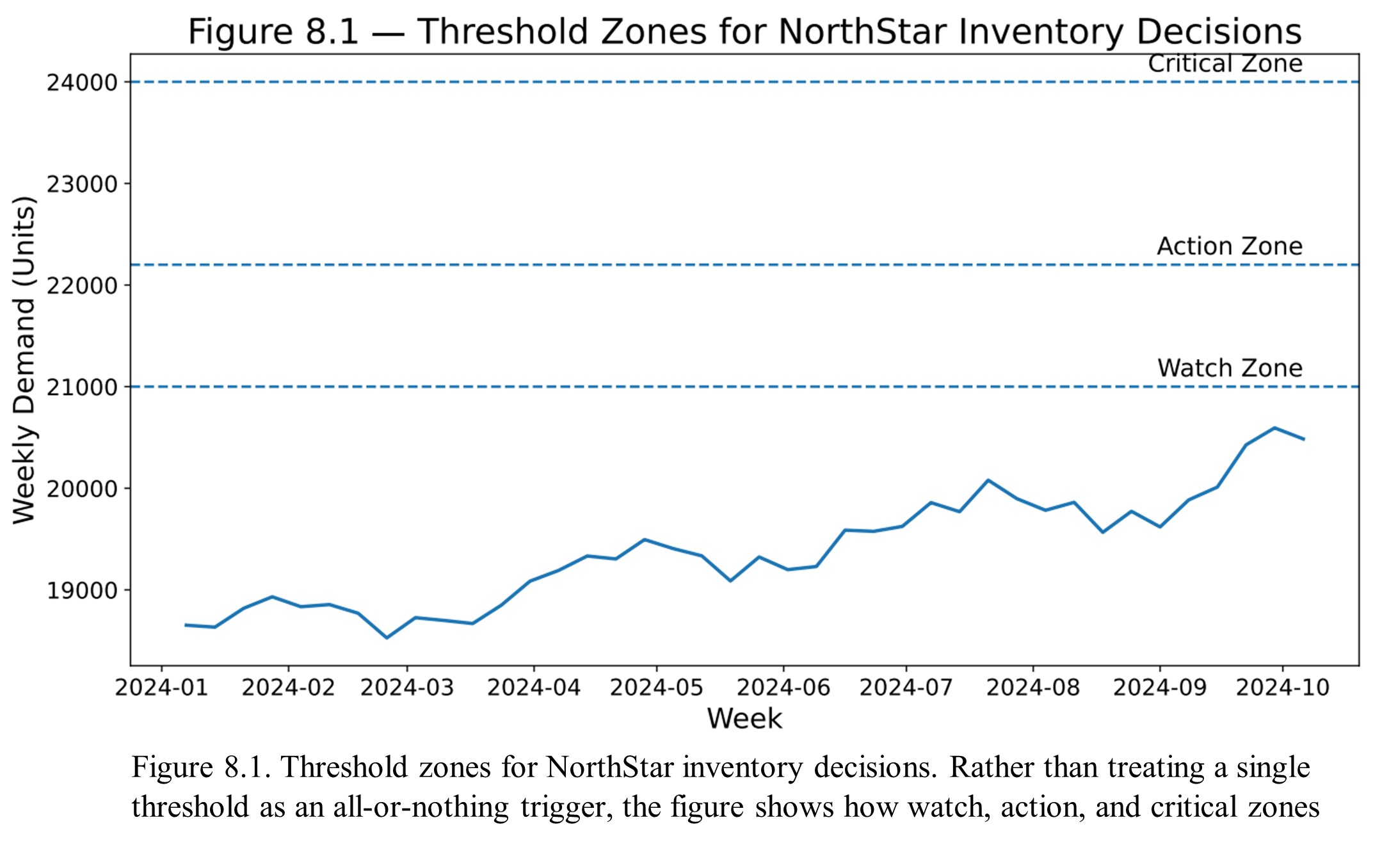
Forecasts describe what might happen.
Thresholds define when that possibility becomes actionable.
For the Everyday Essentials product line, NorthStar defines:
This threshold reflects operational realities:
Thresholds are therefore not arbitrary—they are design choices grounded in system capacity.
Suppose:
A signal-driven lens suggests demand may reach 21,800 within four weeks, with uncertainty bands that could exceed the threshold.
The analyst evaluates:
Rather than treating 22,200 as a hard cutoff, the analyst defines decision zones:
This transforms a threshold from a static number into a contextual decision boundary.
To make thresholds operational, NorthStar establishes explicit trigger rules through cross-functional collaboration:
These statements convert forecasts into clear, accountable actions.
Thresholds are not about precision.
They are about preparedness.
A threshold is a commitment to act before uncertainty becomes failure.
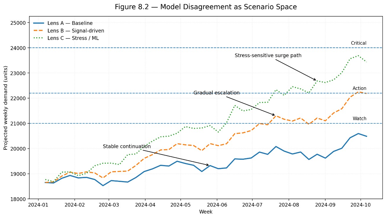
At NorthStar, different models or lenses rarely agree perfectly.
This is not a flaw—it is a feature.
For the same product line:
Each represents a different interpretation of the environment.
Importantly, lenses are not limited to model outputs. They can be constructed from multiple sources:
A forecasting lens is a decision-relevant perspective, not just a statistical projection.
Instead of asking:
Which model is correct?
The analyst asks:
|
Lens |
Scenario |
Business Risk |
|---|---|---|
|
Baseline |
steady demand |
over-preparation |
|
Signal-driven |
gradual rise |
delayed scaling |
|
ML / Surge |
sharp increase |
stockout risk |
Lenses become useful when translated into:
For example:
Agreement can create false confidence.
Diverse lenses create structured awareness.
They do not compete to be right.
They collectively describe what could happen.
At NorthStar, decisions must hold even when forecasts are uncertain.
Strategy A — Wait
Strategy B — Prepare Early
The analyst evaluates:
If stockouts significantly damage revenue and customer trust, early preparation may be preferred, even if the surge is uncertain.
A robust decision:
Robustness reframes decision-making:
Not “What is most likely?”
but “What decision protects us across plausible futures?”
This chapter completes the logic by designing decision systems.
Inputs
Interpretation
Decision Rules
Actions
Governance
Monitoring
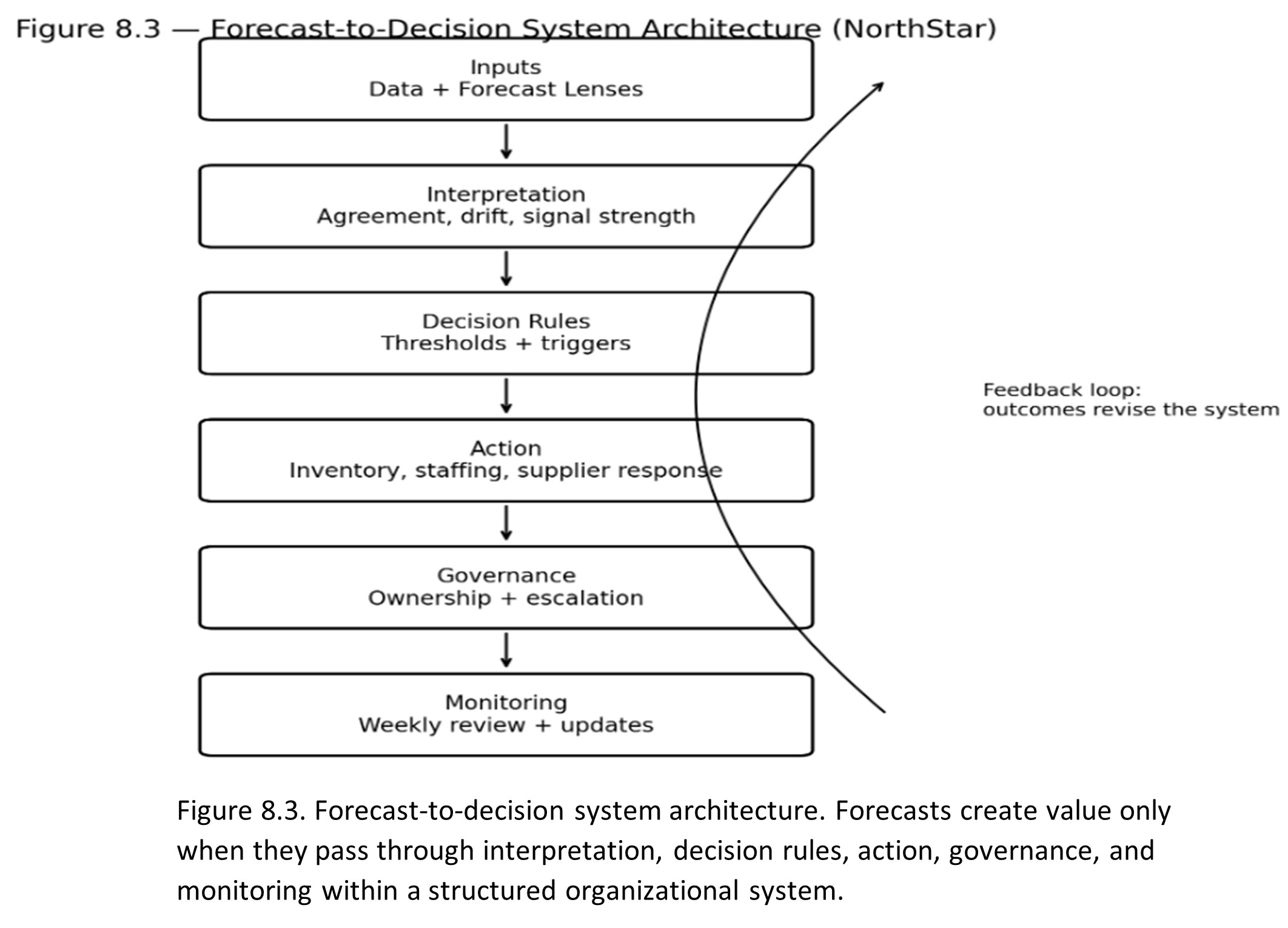
Forecasts generate insight.
Decision systems generate action.
The value of forecasting is realized only when it is embedded in a system that defines:
Forecasting, by design, is not about prediction alone.
It is about structured action under uncertainty.
From Multi-Lens Outputs to Threshold Signals and Governance Logic
This SkillBox develops your ability to transform forecasting outputs into decision-ready signals.
You are not evaluated on model optimization.
You are evaluated on whether you can:
You are supporting NorthStar RetailGroup, which must decide whether to increase inventory and staffing capacity ahead of a potential demand surge in essential goods.
Leadership has defined a supply advisory demand level of 3500 unit per week and a key threshold:
Inventory ratio = 1 – sales/3500 < 20% triggers operational escalation
Your task is to determine:
Use the primary dataset: essentials_sales.csv with variables:
You will construct three forecasting lenses:
Then generate decision-oriented outputs:
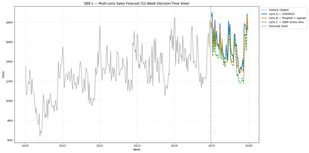
SB8-1: Multi-lens forecast comparison (Decision-Time View)
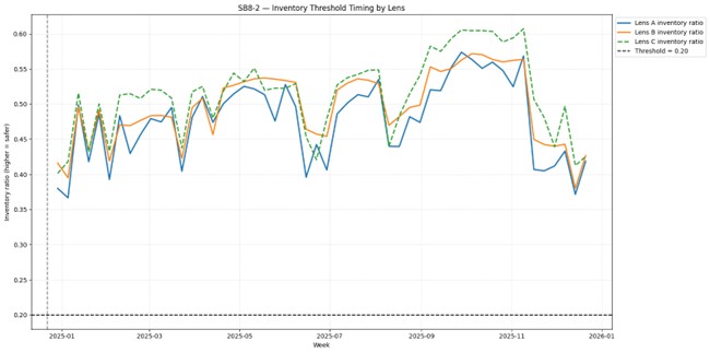
SB8-2: Inventory threshold timing analysis
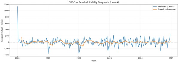
SB8-3: Residual stability diagnostic (Lens A)
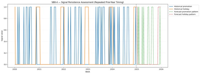
SB8-4: Signal persistence assessment
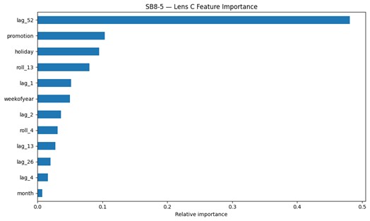
SB8-5: Feature importance (Lens C)
Implementation (Python)
# =========================================================
# SkillBox 8 — Building a Decision-Ready Forecasting System
# NorthStar RetailGroup | 52-week forward forecast
# =========================================================
# Purpose:
# Build three forecasting lenses and convert them into
# threshold-aware inventory signals for decision design.
#
# Lenses:
# Lens A — SARIMAX baseline
# Lens B — Prophet + event signals
# Lens C — GBM stress lens
#
# Decision threshold:
# Inventory ratio < 0.20 triggers operational escalation
#
# Design choice:
# Promotion and holiday indicators in the forecast period
# repeat at the same week positions as in the previous year.
#
# Inventory assumption in this version:
# inventory ratio = 1 - forecasted sales / 3000
#
# Interpretation:
# higher sales -> lower inventory ratio
# higher inventory ratio -> safer
# lower inventory ratio -> more pressure
# =========================================================
import warnings
warnings.filterwarnings("ignore")
import numpy as np
import pandas as pd
import matplotlib.pyplot as plt
from statsmodels.tsa.statespace.sarimax import SARIMAX
from prophet import Prophet
from sklearn.ensemble import GradientBoostingRegressor
# ---------------------------------------------------------
# 0) Load and prepare data
# ---------------------------------------------------------
df = pd.read_csv("essentials_sales.csv")
required_base_cols = ["week", "sales", "promotion", "holiday"]
missing_base = [c for c in required_base_cols if c not in df.columns]
if missing_base:
raise ValueError(f"Missing required columns: {missing_base}")
df["week"] = pd.to_datetime(df["week"])
df = df.sort_values("week").reset_index(drop=True)
if "week_index" not in df.columns:
df["week_index"] = np.arange(1, len(df) + 1)
df["sales"] = pd.to_numeric(df["sales"])
df["promotion"] = pd.to_numeric(df["promotion"])
df["holiday"] = pd.to_numeric(df["holiday"])
inventory_threshold = 0.20
inventory_divisor = 3000.0
print("Columns available:", list(df.columns))
print("\nData preview:")
print(df.head())
# ---------------------------------------------------------
# 1) Forecast horizon = 52 weeks
# ---------------------------------------------------------
h = 52
if len(df) < 52:
raise ValueError("Need at least 52 weeks of history for this SkillBox.")
if len(df) < 104:
print("\nWarning: fewer than 104 weeks of history. Annual seasonality may be less stable.")
last_week = df["week"].iloc[-1]
future_weeks = pd.date_range(start=last_week + pd.Timedelta(weeks=1), periods=h, freq="W")
# ---------------------------------------------------------
# 2) Repeat promotion/holiday timing from previous year
# ---------------------------------------------------------
last_year_events = df[["promotion", "holiday"]].iloc[-52:].reset_index(drop=True)
future_exog = pd.DataFrame({
"week": future_weeks,
"promotion": last_year_events["promotion"].values,
"holiday": last_year_events["holiday"].values,
"week_index": np.arange(
df["week_index"].iloc[-1] + 1,
df["week_index"].iloc[-1] + h + 1
)
})
# ---------------------------------------------------------
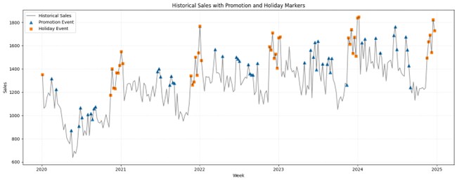
# 3) Historical plot with event markers
# ---------------------------------------------------------
plt.figure(figsize=(15, 6))
plt.plot(df["week"], df["sales"], label="Historical Sales", color="black", alpha=0.45, lw=1.3)
promo = df[df["promotion"] == 1]
holiday = df[df["holiday"] == 1]
plt.scatter(promo["week"], promo["sales"], marker="^", s=45, label="Promotion Event")
plt.scatter(holiday["week"], holiday["sales"], marker="s", s=35, label="Holiday Event")
plt.title("Historical Sales with Promotion and Holiday Markers")
plt.xlabel("Week")
plt.ylabel("Sales")
plt.grid(True, linestyle=":", alpha=0.5)
plt.legend()
plt.tight_layout()
plt.show()
# =========================================================
# LENS A — SARIMAX baseline
# =========================================================
print("\nFitting Lens A — SARIMAX...")
exog_cols = ["promotion", "holiday"]
lensA = SARIMAX(
df["sales"],
exog=df[exog_cols],
order=(1, 1, 1),
seasonal_order=(1, 1, 1, 52),
trend="n",
enforce_stationarity=False,
enforce_invertibility=False
).fit(disp=False)
A_fc = lensA.get_forecast(steps=h, exog=future_exog[exog_cols])
A_mean = np.asarray(A_fc.predicted_mean, dtype=float)
# =========================================================
# LENS B — Prophet + signals
# =========================================================
print("Fitting Lens B — Prophet + signals...")
p_train = df.rename(columns={"week": "ds", "sales": "y"})[
["ds", "y", "promotion", "holiday"]
].copy()
p_future = future_exog.rename(columns={"week": "ds"})[
["ds", "promotion", "holiday"]
].copy()
prophet_model = Prophet(
yearly_seasonality=True,
weekly_seasonality=False,
daily_seasonality=False
)
prophet_model.add_regressor("promotion")
prophet_model.add_regressor("holiday")
prophet_model.fit(p_train)
B_fc = prophet_model.predict(p_future)
B_mean = B_fc["yhat"].values
# =========================================================
# LENS C — GBM stress lens
# =========================================================
print("Fitting Lens C — GBM stress lens...")
def add_features(data):
d = data.copy()
d["month"] = d["week"].dt.month
d["weekofyear"] = d["week"].dt.isocalendar().week.astype(int)
for lag in [1, 2, 4, 13, 26, 52]:
d[f"lag_{lag}"] = d["sales"].shift(lag)
d["roll_4"] = d["sales"].shift(1).rolling(4).mean()
d["roll_13"] = d["sales"].shift(1).rolling(13).mean()
return d
df_gbm = add_features(df)
gbm_features = [
"promotion", "holiday", "month", "weekofyear",
"lag_1", "lag_2", "lag_4", "lag_13", "lag_26", "lag_52",
"roll_4", "roll_13"
]
train_gbm = df_gbm.dropna().copy()
gbm = GradientBoostingRegressor(
n_estimators=400,
learning_rate=0.03,
max_depth=3,
random_state=7
)
gbm.fit(train_gbm[gbm_features], train_gbm["sales"])
# Recursive forecast
gbm_preds = []
gbm_history = df.copy()
for i in range(h):
next_row = future_exog.iloc[[i]].copy()
tmp = pd.concat(
[
gbm_history[["week", "sales", "promotion", "holiday"]],
pd.DataFrame({
"week": next_row["week"].values,
"sales": [np.nan],
"promotion": next_row["promotion"].values,
"holiday": next_row["holiday"].values
})
],
ignore_index=True
)
tmp = add_features(tmp)
x_next = tmp.iloc[-1:][gbm_features]
yhat = float(gbm.predict(x_next)[0])
gbm_preds.append(yhat)
gbm_history = pd.concat(
[
gbm_history,
pd.DataFrame({
"week": next_row["week"].values,
"sales": [yhat],
"promotion": next_row["promotion"].values,
"holiday": next_row["holiday"].values,
"week_index": [next_row["week_index"].values[0]]
})
],
ignore_index=True
)
C_mean = np.array(gbm_preds)
# =========================================================
# 4) Convert forecasted sales into inventory ratios
# =========================================================
# Requested assumption:
# inventory ratio = 1 - forecasted sales / 3000
def to_inventory_ratio(sales_array, divisor=3000.0):
ratio = 1.0 - (np.asarray(sales_array, dtype=float) / divisor)
return np.clip(ratio, 0.0, 1.0)
A_inv = to_inventory_ratio(A_mean, inventory_divisor)
B_inv = to_inventory_ratio(B_mean, inventory_divisor)
C_inv = to_inventory_ratio(C_mean, inventory_divisor)
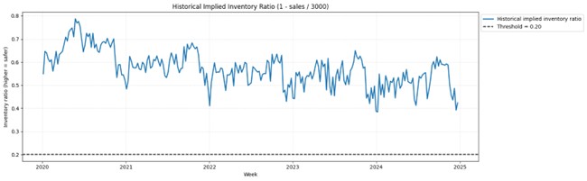
# Historical implied inventory ratio under same assumption
df["inventory_ratio_implied"] = to_inventory_ratio(df["sales"], inventory_divisor)
# =========================================================
# 5) Threshold timing summary
# =========================================================
def first_below(arr, threshold):
idx = np.where(np.asarray(arr) < threshold)[0]
return None if len(idx) == 0 else int(idx[0] + 1)
threshold_table = pd.DataFrame({
"Lens": ["A (SARIMAX)", "B (Prophet+signals)", "C (GBM)"],
"First week inventory ratio < 0.20": [
first_below(A_inv, inventory_threshold),
first_below(B_inv, inventory_threshold),
first_below(C_inv, inventory_threshold)
]
})
print("\nSB8-2 Threshold Timing Table")
print(threshold_table)
# =========================================================
# SB8-1 — Multi-lens sales forecast
# =========================================================
plt.figure(figsize=(16, 8))
plt.plot(df["week"], df["sales"], label="History (Sales)", color="black", alpha=0.45, lw=1.2)
plt.plot(future_weeks, A_mean, label="Lens A — SARIMAX", lw=2.3)
plt.plot(future_weeks, B_mean, label="Lens B — Prophet + signals", lw=2.1)
plt.plot(future_weeks, C_mean, label="Lens C — GBM stress lens", lw=2.0, linestyle="--")
plt.axvline(df["week"].iloc[-1], color="gray", linestyle="--", label="Forecast Start")
plt.title("SB8-1 — Multi-Lens Sales Forecast (52-Week Decision-Time View)")
plt.xlabel("Week")
plt.ylabel("Sales")
plt.legend(loc="upper left", bbox_to_anchor=(1, 1))
plt.grid(True, linestyle=":", alpha=0.6)
plt.tight_layout()
plt.show()
# =========================================================
# SB8-2 — Inventory threshold timing plot
# =========================================================
plt.figure(figsize=(16, 8))
plt.plot(future_weeks, A_inv, label="Lens A inventory ratio", lw=2.2)
plt.plot(future_weeks, B_inv, label="Lens B inventory ratio", lw=2.0)
plt.plot(future_weeks, C_inv, label="Lens C inventory ratio", lw=2.0, linestyle="--")
plt.axhline(inventory_threshold, color="black", linestyle="--", label="Threshold = 0.20")
plt.axvline(df["week"].iloc[-1], color="gray", linestyle="--")
plt.title("SB8-2 — Inventory Threshold Timing by Lens")
plt.xlabel("Week")
plt.ylabel("Inventory ratio (higher = safer)")
plt.legend(loc="upper left", bbox_to_anchor=(1, 1))
plt.grid(True, linestyle=":", alpha=0.6)
plt.tight_layout()
plt.show()
# =========================================================
# SB8-3 — Residual stability diagnostic (Lens A)
# =========================================================
fit_A = np.asarray(lensA.fittedvalues, dtype=float)
n = min(len(df["sales"]), len(fit_A))
resid_A = df["sales"].iloc[-n:].to_numpy(dtype=float) - fit_A[-n:]
resid_A = pd.Series(resid_A, index=df["week"].iloc[-n:])
roll_mean = resid_A.rolling(8).mean()
plt.figure(figsize=(14, 5))
plt.plot(resid_A.index, resid_A.values, label="Residuals (Lens A)")
plt.plot(roll_mean.index, roll_mean.values, label="8-week rolling mean", lw=2)
plt.axhline(0, linestyle="--", color="gray")
plt.title("SB8-3 — Residual Stability Diagnostic (Lens A)")
plt.xlabel("Week")
plt.ylabel("Residual (Actual − Fitted)")
plt.legend()
plt.grid(True, linestyle=":", alpha=0.5)
plt.tight_layout()
plt.show()
# =========================================================
# SB8-4 — Signal persistence panel
# =========================================================
plt.figure(figsize=(16, 6))
plt.plot(df["week"], df["promotion"], label="Historical promotion", lw=1.8)
plt.plot(df["week"], df["holiday"], label="Historical holiday", lw=1.8)
plt.plot(future_weeks, future_exog["promotion"], label="Forecast promotion pattern", linestyle="--")
plt.plot(future_weeks, future_exog["holiday"], label="Forecast holiday pattern", linestyle="--")
plt.axvline(df["week"].iloc[-1], linestyle="--", color="gray")
plt.title("SB8-4 — Signal Persistence Assessment (Repeated Prior-Year Timing)")
plt.xlabel("Week")
plt.ylabel("Signal value")
plt.legend(loc="upper left", bbox_to_anchor=(1, 1))
plt.grid(True, linestyle=":", alpha=0.5)
plt.tight_layout()
plt.show()
# =========================================================
# SB8-5 — Feature importance
# =========================================================
importances = pd.Series(gbm.feature_importances_, index=gbm_features).sort_values(ascending=False)
print("\nSB8-5 Feature Importance (Top 12)")
print(importances.head(12))
plt.figure(figsize=(10, 6))
importances.head(12).sort_values().plot(kind="barh")
plt.title("SB8-5 — Lens C Feature Importance")
plt.xlabel("Relative importance")
plt.tight_layout()
plt.show()
# =========================================================
# Optional historical implied inventory plot
# =========================================================
plt.figure(figsize=(16, 5))
plt.plot(df["week"], df["inventory_ratio_implied"], label="Historical implied inventory ratio", lw=2)
plt.axhline(inventory_threshold, color="black", linestyle="--", label="Threshold = 0.20")
plt.title("Historical Implied Inventory Ratio (1 - sales / 3000)")
plt.xlabel("Week")
plt.ylabel("Inventory ratio (higher = safer)")
plt.legend(loc="upper left", bbox_to_anchor=(1, 1))
plt.grid(True, linestyle=":", alpha=0.6)
plt.tight_layout()
plt.show()
# =========================================================
# Export reporting tables
# =========================================================
forecast_table = pd.DataFrame({
"week": future_weeks,
"A_sales": A_mean,
"B_sales": B_mean,
"C_sales": C_mean,
"A_inventory_ratio": A_inv,
"B_inventory_ratio": B_inv,
"C_inventory_ratio": C_inv
})
forecast_table.to_csv("skillbox8_forecast_outputs.csv", index=False)
threshold_table.to_csv("skillbox8_threshold_timing.csv", index=False)
print("\nSaved output files:")
print("- skillbox8_forecast_outputs.csv")
print("- skillbox8_threshold_timing.csv")
Implementation (R)
Due to space limitations, the R code is not provided here. As an AI-supported learning exercise, interested readers may use a tool such as ChatGPT to translate the provided Python code into R and then learn the R workflow by reverse-engineering the generated code and outputs.
👉 Interpretation
👉 Interpretation
👉 Interpretation
👉 Interpretation
👉 Interpretation
👉 Interpretation
Your analysis must clarify this tradeoff explicitly.
Treating models as competitors instead of evidence sources.
A forecast becomes valuable only when it changes when and how you act, or triggers new questions.
You will now use AI to interpret disagreement and design decision logic without surrendering judgment.
Using AI as a Learning and Thinking Partner
This LearningLab reinforces the analytical ideas introduced in the SkillBox by using AI as both a learning partner and a thinking partner, rather than a modeling shortcut.
The objective is to:
This LearningLab reinforces:
In the preceding SkillBox, you constructed and compared multiple forecasting lenses (e.g., baseline, signal-driven, and machine learning perspectives). You observed how the same data can produce different forward-looking signals depending on modeling assumptions and structure.
This LearningLab introduces the next step: using AI to deepen understanding, extend analysis, and explore decision implications of these differences.
AI is used here to:
AI responses should be treated as hypotheses, not conclusions.
NorthStar analysts have developed three forecasting lenses for weekly demand:
However, the forecasts do not fully agree.
Key questions include:
To support this process, analysts use AI not to generate answers, but to expand and challenge their reasoning about how forecasts should inform decisions.
You will engage with AI at three levels:
Reinforce → Extend → Explore
Work through the modes in order.
Purpose
Confirm and strengthen your understanding of core concepts from this chapter, especially multi-lens forecasting and decision thresholds.
AI Role
Suggested Prompts
“Key Concepts from Chapter 8.
Outcome
“I understand how multiple forecasts represent different perspectives and why they are useful.”
Purpose
Extend your analytical capability by connecting multi-lens forecasting to evaluation, uncertainty, and system design.
AI Role
Suggested Prompts
Outcome
“I can analyze and compare multiple forecast outputs and connect them to evaluation and uncertainty.”
Purpose
Develop judgment by connecting multi-lens forecasting to real decision systems, including risk, timing, and organizational impact.
AI Role
Suggested Prompts
Outcome
“I understand how forecasting systems translate into real decisions under uncertainty.”
After completing all three modes:
The goal is to evaluate reasoning, not outsource it.
Prepare a short written summary (200–300 words) describing:
You must:
AI expands analytical range but does not replace analytical responsibility.
AI can:
• accelerate explanation
• broaden analytical exploration
• surface alternative interpretations of forecast disagreement
But it cannot:
• ensure correctness
• replace contextual judgment
• assume responsibility for decisions
Insight: Multi-lens forecasting expands visibility—but decision quality depends on how those lenses are governed.
The next step is not further analysis—but decision system design.
How should multiple forecasts be translated into:
• thresholds,
• escalation rules, and
• operational actions?
The DesignStudio will move from:
understanding → reasoning → decision system design
Excellent—Chapter 8 is the capstone integration layer, where everything shifts decisively from:
forecasting models → forecasting systems → decision design
So the LearningLab must elevate from comparison (Ch7) to action design (Ch8).
Below is the fully polished, publisher-ready LearningLab 8, tightly aligned with:
To design a governed decision system using forecasts.
NorthStar must decide whether to:
Design a system that determines:
Design a decision system addressing:
2–3 page decision system design
Good decisions are not optimized for one future—they are designed for many.
You will now apply your system under ambiguity.
Committing capacity decisions under uncertain demand
A regional hospital network uses weekly patient-volume forecasts to plan staffing, bed capacity, and critical resource allocation (e.g., ICU beds, ventilators, and emergency department coverage).
Historically, planning has relied on a single baseline forecast derived from seasonal patterns and long-term trends.
As the hospital enters a period of heightened uncertainty—driven by early indicators of a potential respiratory illness surge—analysts have developed three forecasting lenses:
The projections are close and partially overlapping, with no definitive indication that a surge will occur. However, recent developments—including rising case counts in neighboring regions and increased emergency visits—suggest that the stress scenario is plausible, even if not the most likely.
Hospital leadership has asked your team to prepare a recommendation assuming the surge scenario could materialize, given the high consequences of under-preparation.
Two weekly planning cycles remain before staffing schedules and resource allocations must be finalized.
If the surge (stress) scenario were to occur, what actions should the hospital take now to ensure readiness—without overcommitting resources prematurely?
Assume the surge scenario is credible, though uncertain.
As a cross-functional decision group (clinical operations, staffing, and administration), answer the following:
If the surge scenario materializes:
Focus on timing and system capacity, not just volume.
Compare the risks of:
Which risk is more severe in this context, and why?
What actions should be taken now, before full confirmation?
Examples may include:
Your recommendations should balance:
What signals should trigger:
Be explicit:
How would you communicate your plan to hospital leadership?
Your message should:
Write a short executive note recommending:
In high-stakes environments such as healthcare, the cost of under-preparation is often nonlinear and irreversible.
Decision-making is therefore not based solely on what is most likely, but on what is plausible and consequential.
Effective organizations do not wait for certainty.
They design conditional actions that protect against high-impact outcomes.
Forecasts do not create decisions—systems do.
When models disagree, they reveal structure in uncertainty that must be interpreted, not resolved.
A well-designed decision system transforms that uncertainty into timely, accountable, and defensible action.
NorthStar RetailGroup has now moved from forecasting to decision system design. Instead of relying on a single demand projection, the organization has implemented a multi-lens monitoring system anchored by thresholds and supported by signal diagnostics. Inventory decisions are no longer reactive; they are triggered by structured conditions tied to risk and lead time. As a result, NorthStar improves not only responsiveness but also accountability—ensuring that decisions remain coherent even when forecasts diverge.
Student Guidance
Even the most carefully designed decision system faces a deeper challenge:
What happens when the environment itself changes?
When relationships between variables shift, signals become unstable, and past patterns no longer apply, decision systems must do more than respond—they must adapt.
In the next chapter, we extend Forecast-by-Design into organizational learning systems, where forecasts, decisions, and feedback loops evolve together over time.
The question is no longer how to design decisions—
but how to design systems that learn from their own decisions.
CAPSTONE PROJECT — FORECAST BY DESIGN
Designing a Healthcare Capacity Decision System Under Uncertainty
Core Objective
Design a forecast-driven decision system for hospital capacity planning that enables leaders to act:
What Makes This a Capstone
In Chapter 8, you worked in a guided environment (NorthStar).
In this capstone:
Your task is not to apply a method.
Your task is to design a decision system from scratch.
Capstone Philosophy
This is NOT:
This IS:
Models don’t decide—systems do.
You are advising a regional hospital network.
Leadership must decide:
Should we activate surge capacity protocols within the next 4–8 weeks?
Operational Decisions Include
Decision Stakes (Asymmetric Risk)
|
Action Timing |
Consequence |
|
Too early |
high cost, disruption |
|
Too late |
patient risk, system overload |
Your Role
You are the Decision Analytics Team.
You must provide:
III. Dataset
File
healthcare_capacity_weekly.csv
Variables
Data Characteristics
You are expected to construct multiple analytical perspectives, but:
You are NOT required to build complex models
Required Lenses (Conceptual, not rigid)
You must include:
These do NOT need to be:
They must be:
You must design a Healthcare Capacity Decision System that includes:
Define at least two thresholds, such as:
Define:
What combination of signals triggers action?
Example:
Estimate:
Define:
Define:
Format Options
Required Sections
VII. Thinking Requirements (MANDATORY)
Your work MUST demonstrate:
|
Stage |
Evidence |
|
Observe |
problem framing |
|
Understand |
structure + signals |
|
Practice |
analytical outputs |
|
Reason |
uncertainty interpretation |
|
Design |
thresholds + system |
|
Decide |
recommendation |
|
Integrate |
coherence |
|
Consolidate |
reflection |
|
Continue |
limitations |
VIII. Evaluation Rubric (100 Points)
Grade A
Grade B
Grade C
Allowed:
Not Allowed:
Required Disclosure
Students must include:
XIII. Capstone Design Insight
The purpose of this capstone is not to predict hospital demand.
It is to design a system that ensures patients are protected even when predictions are uncertain.

