Designing Visible Temporal Structure
Forecasting with Trend and Seasonality as Explicit Components
When organizations begin using forecasts to guide staffing, budgets, inventory, and operating commitments, they can no longer treat time patterns as vague impressions. A rising line on a chart is not enough. Leaders need to know whether projected growth reflects a durable trend, a recurring seasonal cycle, or a temporary fluctuation that should not be turned into a costly commitment.
That is the central challenge of this chapter. In earlier chapters, we learned how to smooth noisy series and how to separate time-based patterns for interpretation. Here, the goal changes: visible temporal structure must now be represented in a way that can support projection, accountability, and defensible planning. The question is no longer simply What patterns do we see? It becomes Which visible patterns should be carried forward, and on what grounds?
This chapter focuses on the first major forecasting design path: explicit structure. In this approach, trend and seasonality are treated as visible components that can be separated, interpreted, projected, and recombined. This makes assumptions easier to explain, easier to challenge, and easier to connect to decisions. It also creates a new responsibility: if the projected structure is wrong, the forecast may remain elegant while the decision fails.
Chapters 2 and 3 established an essential discipline: before forecasting, analysts must first learn to see structure in time. Smoothing helped reduce noise so that short-term movement could be interpreted more responsibly. Decomposition then separated layered temporal patterns so that long-term direction, recurring rhythm, and irregular variation would not be confused with one another. Those chapters were primarily interpretive. They helped us understand time-ordered data before asking it to support forward-looking commitments.
Chapter 4 moves from interpretation to representation. Once a forecast begins influencing labor plans, inventory targets, budget commitments, promotional calendars, or service capacity, pattern recognition alone is no longer enough. The organization must decide which visible structures in the historical series are persistent enough to project into the future. That is a design decision, not a purely technical one.
This chapter therefore introduces forecasting with visible temporal structure. The focus is on trend and seasonality as explicit components that can be estimated separately and then projected forward in a transparent way. The representative method is STL-based explicit-structure forecasting, not because it is the only approach available, but because it clearly illustrates the logic of making temporal assumptions visible. In this framework, forecasting becomes a disciplined statement about what the organization believes will persist, what it expects to repeat, and what it is willing to treat as uncertainty.
This emphasis is fully consistent with the philosophy of this book: forecasting is a decision-support system, not a prediction contest. The aim is not to produce a number that looks sophisticated. The aim is to produce a forecast whose assumptions can be interpreted, questioned, communicated, and used responsibly.
This chapter follows the Forecast-by-Design reasoning progression:
Observe → Understand → Practice → Reason → Design → Decide → Integrate → Consolidate → Continue
You will begin by
After completing this chapter, students should be able to:
When forecasts guide real decisions, how should visible temporal structure—especially trend and seasonality—be represented so that assumptions remain interpretable, accountable, and decision-useful over time?
When you manage electricity demand for more than 30 million people, forecasting is not just about producing the latest number. It is about defending the assumptions that justify plant schedules, maintenance windows, capacity commitments, and regulatory decisions. At Tokyo Electric Power Company (TEPCO), a forecasting error is never just a statistical miss. It can cascade into costly overcapacity, strained infrastructure, or heightened scrutiny from regulators and the public.
For years, the organization relied heavily on tools that helped analysts respond to short-term demand movement: smoothing procedures, rolling averages, and expert overlays informed by weather expectations. Those tools were useful when the main task was operational responsiveness. They helped calm noise and track short-horizon variation. But over time, Japan’s energy environment became harder to read. Energy-efficient homes changed consumption patterns. Industrial users shifted production schedules. Climate volatility altered seasonal behavior. Demand still moved in rhythms, but those rhythms were no longer as easy to interpret from the aggregate series alone.
The problem was not that the organization lacked forecasts. The problem was that leaders could no longer tell what visible movement in the series actually meant. Was a rising summer profile evidence of sustained growth? Was it just a stronger seasonal peak? Was a recent flattening a structural shift in demand, or merely a temporary interruption? The smoothed forecasts produced useful signals, but they did not clearly separate long-term movement from recurring seasonal behavior.
That distinction mattered. If planners interpreted a seasonal upswing as durable growth, they risked locking in excessive capacity. If they dismissed a changing trend as mere volatility, they risked underpreparing for structural demand shifts. In both cases, the organization would still have a forecast—but not one grounded in interpretable structure.
This is the setting in which visible temporal structure becomes a design problem. Forecasts are more trustworthy when trend and seasonality are made explicit rather than left buried inside the aggregate series. Once those components are separated, managers can ask better questions: Which part of projected demand reflects long-term movement? Which part reflects recurring seasonal rhythm? Which part should be treated as uncertainty rather than projected confidently into the future?
This chapter focuses on that discipline. It shows how trend and seasonality can be represented explicitly so that forecasts become easier to interpret, easier to communicate, and easier to use responsibly. It also sets up the next chapter’s unresolved challenge: visible structure is not the whole story, because some forms of temporal dependence cannot be seen directly at all.
In Chapters 2 and 3, the analyst’s task was mainly observational and interpretive. Smoothing helped reveal signal in noisy movement. Decomposition helped separate long-term direction from recurring rhythm and irregular variation. Those steps improved understanding, but they did not yet require the analyst to commit to a forecast design.
Chapter 4 changes that. Once a forecast influences budgets, headcount plans, service capacity, or working capital, pattern recognition must become representation. The organization is no longer asking only what the historical series looks like. It is asking which visible structures should be projected forward and which should be treated cautiously.
An executive analogy helps here. Exploratory analysis is like reviewing a dashboard before a meeting: it helps you notice movement, compare patterns, and raise questions. Forecast design is closer to approving a plan: once numbers enter a budget or staffing commitment, the assumptions behind them become organizationally consequential. What was once an observation now becomes a commitment.
This is why explicit structure matters. If trend and seasonality remain blended together in a single projected series, leaders may agree on the forecast while disagreeing silently on what it means. One team may interpret the projection as durable growth. Another may interpret the same number as temporary seasonality. The forecast becomes fragile not because the number is wrong, but because the assumptions are hidden.
The central design idea of this chapter is therefore simple but powerful: make visible structure visible in the forecast itself. This is the first major application of the chapter memory anchor:
Structure → Behavior → Trust
If structure is represented clearly, forecast behavior becomes more interpretable. When forecast behavior is interpretable, trust becomes easier to build and maintain. And when trust is stronger, decisions become more accountable.
Explicit-structure forecasting treats visible temporal patterns as separate forecasting objects. Instead of asking a single model to absorb all time-based behavior at once, the analyst separates the series into components, projects the components that appear persistent, and then recombines them into a forecast.
In additive form, the observed series can be represented as:
where:
For forecasting h steps ahead of time point t, the logic becomes:
The remainder Rₜ is not projected as though it were a stable pattern. It is treated as uncertainty around the structural forecast.
The point of this representation is not mathematical elegance. The point is managerial clarity. Trend tells a story about persistent movement. Seasonality tells a story about recurring rhythm. Remainder tells a story about what should not be overinterpreted. Once these are separated, the organization can debate assumptions more productively.
Consider NorthStar RetailGroup. Suppose weekly unit sales for an everyday essentials category rise every late summer and fall after promotional intensity declines. If that recurring pattern is not separated from the broader direction of the series, leaders may misread predictable seasonal strength as evidence of permanent demand growth. Finance may support tighter cost controls and higher revenue expectations. Operations may overcommit capacity. Marketing may assume a campaign permanently lifted demand when it mainly shifted timing. Explicit structure reduces that risk by making the underlying assumptions inspectable.
This is not merely a convenience. It is a governance discipline. Models don’t decide—systems do. Explicit structure helps the system see what kind of movement it is responding to.
This chapter uses STL (Seasonal-Trend decomposition using Loess) as the representative method for explicit visible structure. STL is valuable here not because it is the only decomposition method, but because it makes the chapter’s design logic especially clear.
STL separates a series into trend, seasonality, and remainder using flexible smoothing rather than rigid pre-specified formulas. That flexibility matters because visible structure often evolves. Trend is rarely perfectly linear. Seasonal patterns are rarely identical year after year. STL gives analysts a way to estimate visible structure without pretending that the system is more rigid than it really is.
Its business value lies in interpretability. Leaders can see which part of the forecast reflects long-term movement and which part reflects expected repetition. That visibility supports communication, challenge, and accountability.
At the same time, explicit structure introduces risk. If the analyst projects a trend that is already weakening, the forecast may carry forward a pattern that no longer holds. If the analyst assumes seasonal stability in a system whose operating calendar has changed, the forecast may repeat a rhythm that is no longer reliable. This is the chapter’s error lens: visible structure can be interpreted clearly and still be projected poorly.
So the question is not whether explicit structure is good or bad. The question is whether the visible structure is plausible enough to support the decision at hand.
Not every time series behaves the same way as its level changes. In some settings, seasonal variation remains roughly stable even as the overall level shifts. In others, the size of the seasonal swings grows along with the level of the series. That distinction matters because it affects how visible structure should be represented.
An additive view assumes that the absolute size of seasonal movement remains roughly constant across time:
A multiplicative view assumes that seasonal movement is proportional to the level of the series:
In practice, analysts often use a logarithmic transformation to convert proportional movement into additive structure on the transformed scale:
For this chapter, the operational focus remains on additive structure because it supports the clearest introduction to explicit forecasting design. The deeper issues of transformation, validation, and uncertainty are taken up later when diagnostic tools are more fully developed.
The main student-facing point is straightforward: the analyst is not just identifying visible structure, but deciding how that structure should be represented. Different representations imply different assumptions about persistence and scale. Those assumptions should be chosen because they improve decision usefulness, not because they make formulas look more advanced.
Forecasting with visible structure can be understood as a sequence of disciplined analytical questions.
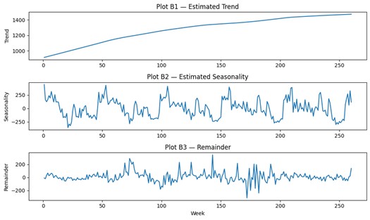
Step 1 — Estimate the visible components
The series is separated into estimated trend, seasonality, and remainder:
At this stage, the goal is not perfection. The goal is a meaningful separation between persistent visible movement and variation that should not be projected confidently.
For readers who are curious about how these components are estimated, an optional AI tool and sample prompt (e.g., “Illustrate the specific formulas used to estimate each STL component”) are useful. This exploration is intended to build intuition and transparency, not to require implementation or technical execution. Readers may engage with these details to deepen understanding, but doing so is not necessary for applying STL effectively in managerial or decision-oriented contexts.
Step 2 — Evaluate component plausibility
Before projecting anything, the analyst should ask:
This stage matters because explicit forecasting can fail gracefully in appearance while failing seriously in meaning. A smooth trend line can look convincing even when it does not fit the business context.
Step 3 — Project the trend
Once the trend is deemed plausible, it is extended into the forecast horizon based on a transparent continuation rule. The purpose is not to guess a dramatic future change. It is to make the continuity assumption visible: recent long-term movement is being carried forward unless there is reason not to do so.
Step 4 — Extend seasonality
Seasonality is projected by repeating the estimated cycle over the forecast horizon:
where s is the seasonal period (e.g., 52 for weekly data with annual seasonality).
This assumes that the timing and shape of the recurring pattern remain stable enough to matter.
Step 5 — Recombine the projected components
The forecast is formed by recombining projected trend and seasonality:
The remainder is not forecast as if it were a reliable driver. Instead, it is derived for the observed time period as:
It remains a source of uncertainty around the structural projection.
This workflow embodies the chapter’s design logic. Visible structure is separated so that it can be interpreted. Interpreted structure is projected so that it can support action. But projected structure must still be challenged, because transparency is not the same as truth.
Explicit structure helps organizations ask better questions.
Suppose NorthStar RetailGroup is preparing a quarterly inventory and staffing plan for an everyday essentials category. A projected rise in weekly unit sales could mean at least three different things:
These interpretations lead to different decisions. Durable trend growth might justify permanent staffing or supplier negotiations. Seasonal movement might justify temporary labor, timed replenishment, and promotional support. Irregular movement might justify caution rather than expansion.
Without explicit structure, these possibilities remain blended. Teams may act on the same forecast number while carrying very different beliefs about what it means. Explicit decomposition reduces that ambiguity.
This is why the chapter emphasizes decision stakes. If visible structure is misread, decisions can become expensive quickly. Treating seasonality as trend may create overcommitment. Treating trend as seasonality may create underinvestment. Treating structural movement as noise may delay needed action. The analytical task is therefore inseparable from decision design.
It is helpful to contrast this chapter’s approach with what students learned earlier.
Smoothing in Chapter 2 was mainly about creating a stable signal for near-term interpretation. It was useful when managers needed faster sensemaking and not necessarily a fully articulated forward-looking structure. Decomposition in Chapter 3 clarified how multiple patterns coexist in a series, especially for interpretation and communication.
Chapter 4 goes further. It asks the analyst to take visible structure seriously enough to project it. That is a stronger commitment. Once a trend is carried into the forecast horizon and a seasonal cycle is repeated into future periods, the analyst is no longer just describing the past. The analyst is designing what kind of continuity the organization is willing to believe.
That is the key contrast:
This is the chapter’s central conceptual move.
Visible temporal structure is powerful, but it is not complete. Some forms of time dependence are not easily seen by inspection or decomposition. A forecast may look reasonable at the component level and still miss how the series depends on its own recent history. It may represent visible trend and seasonality clearly while failing to capture lingering dependence, serial error patterns, or hidden memory.
That limitation is not a flaw in the chapter. It is the bridge to the next one.
Chapter 4 establishes the logic of forecasting when structure is visible and interpretable. Chapter 5 asks what happens when dependence matters but cannot be read directly from the components. In other words, this chapter teaches how to forecast when time shows its structure openly. The next chapter begins where openness ends.
From explicit components to a decision-ready forecast
This SkillBox develops hands-on analytical capability with explicit visible-structure forecasting . You will separate weekly sales into trend and seasonality, project each component with transparent rules, and recombine them into a forecast that can be interpreted and challenged in a business setting.
NorthStar RetailGroup is preparing a 26-week planning cycle for its Everyday Essentials category. Merchandising, inventory planning, and store operations need a forecast that distinguishes durable movement from recurring calendar rhythm. The point is not just to produce a number, but to show what the number assumes.
Primary dataset: essentials_sales_lite.csv
This chapter continues the required primary dataset so that the analytical change reflects the forecasting design rather than a change in data context.
If NorthStar interprets recurring seasonal demand as permanent growth, it may overcommit inventory, labor, and vendor contracts. If it treats genuine trend growth as temporary seasonality, it may underprepare and lose availability during critical weeks.
You will:
Python
# SkillBox 4 (Python): Explicit visible-structure forecasting with STL
import pandas as pd
import numpy as np
import matplotlib.pyplot as plt
from statsmodels.tsa.seasonal import STL
# Load primary dataset
df = pd.read_csv("essentials_sales_lite.csv")
time_col = "week_index" if "week_index" in df.columns else None
x = df[time_col] if time_col else np.arange(1, len(df) + 1)
y = df["sales"].astype(float)
# Plot A — Original series
plt.figure(figsize=(10, 4))
plt.plot(x, y)
plt.title("Plot A — Weekly Unit Sales (Original Series)")
plt.xlabel("Week")
plt.ylabel("Units Sold")
plt.show()
# STL decomposition
SEASONAL_PERIOD = 52
stl = STL(y, period=SEASONAL_PERIOD, robust=True)
res = stl.fit()
trend = res.trend
seasonal = res.seasonal
remainder = res.resid
# Plot B — Components
plt.figure(figsize=(10, 6))
plt.subplot(3, 1, 1)
plt.plot(x, trend)
plt.title("Plot B1 — Estimated Trend")
plt.ylabel("Trend")
plt.subplot(3, 1, 2)
plt.plot(x, seasonal)
plt.title("Plot B2 — Estimated Seasonality")
plt.ylabel("Seasonality")
plt.subplot(3, 1, 3)
plt.plot(x, remainder)
plt.title("Plot B3 — Remainder")
plt.xlabel("Week")
plt.ylabel("Remainder")
plt.tight_layout()
plt.show()
# Forecast horizon
H = 26
last_week = int(x.iloc[-1]) if time_col else len(df)
future_x = np.arange(last_week + 1, last_week + H + 1)
# Project trend using recent slope
K = min(12, len(trend) - 1)
trend_slope = (trend.iloc[-1] - trend.iloc[-(K+1)]) / K
trend_future = trend.iloc[-1] + trend_slope * np.arange(1, H + 1)
# Repeat seasonal template
season_template = seasonal.iloc[-SEASONAL_PERIOD:].to_numpy()
season_future = np.array([season_template[i % SEASONAL_PERIOD] for i in range(H)])
# Recombine
yhat_future = trend_future + season_future
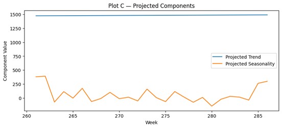
# Plot C — Projected components
plt.figure(figsize=(10, 4))
plt.plot(future_x, trend_future, label="Projected Trend")
plt.plot(future_x, season_future, label="Projected Seasonality")
plt.title("Plot C — Projected Components")
plt.xlabel("Week")
plt.ylabel("Component Value")
plt.legend()
plt.show()
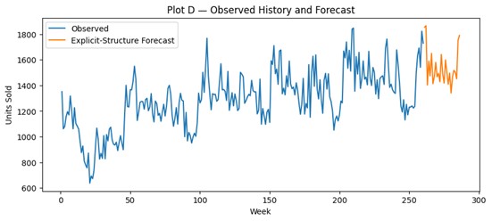
# Plot D — Recombined forecast
plt.figure(figsize=(10, 4))
plt.plot(x, y, label="Observed")
plt.plot(future_x, yhat_future, label="Explicit-Structure Forecast")
plt.title("Plot D — Observed History and Forecast")
plt.xlabel("Week")
plt.ylabel("Units Sold")
plt.legend()
plt.show()
# Forecast breakdown table
out = pd.DataFrame({
"week_index": future_x,
"trend_forecast": trend_future,
"season_forecast": season_future,
"sales_forecast": yhat_future
})
print(out.head(10))
R
# SkillBox 4 (R): Explicit visible-structure forecasting with STL

df <- read.csv("essentials_sales_lite.csv", stringsAsFactors = FALSE)

if ("week_index" %in% names(df)) {
  x <- df$week_index
} else {
  x <- 1:nrow(df)
}

y <- as.numeric(df$sales)

# Plot A — Original series
plot(x, y, type="l",
     main="Plot A — Weekly Unit Sales (Original Series)",
     xlab="Week", ylab="Units Sold")

# STL decomposition
SEASONAL_PERIOD <- 52
y_ts <- ts(y, frequency = SEASONAL_PERIOD)
fit <- stl(y_ts, s.window="periodic", robust=TRUE)

trend <- fit$time.series[, "trend"]
seasonal <- fit$time.series[, "seasonal"]
remainder <- fit$time.series[, "remainder"]

# Plot B — Components
plot(fit, main="Plot B — STL Components")

# Forecast horizon
H <- 26
future_x <- (max(x) + 1):(max(x) + H)

# Project trend
K <- min(12, length(trend) - 1)
trend_slope <- (trend[length(trend)] - trend[length(trend)-K]) / K
trend_future <- trend[length(trend)] + trend_slope * (1:H)

# Repeat seasonal template
season_template <- tail(seasonal, SEASONAL_PERIOD)
season_future <- sapply(1:H, function(i) season_template[((i - 1) %% SEASONAL_PERIOD) + 1])

# Recombine
yhat_future <- trend_future + season_future

# Plot C — Projected components
plot(future_x, trend_future, type="l",
     main="Plot C — Projected Components",
     xlab="Week", ylab="Component Value")
lines(future_x, season_future, lty=2)
legend("topleft",
       legend=c("Projected Trend", "Projected Seasonality"),
       lty=c(1,2), bty="n")

# Plot D — Recombined forecast
plot(x, y, type="l",
     main="Plot D — Observed History and Forecast",
     xlab="Week", ylab="Units Sold")
lines(future_x, yhat_future, lty=2)
legend("topleft",
       legend=c("Observed", "Explicit-Structure Forecast"),
       lty=c(1,2), bty="n")

# Forecast breakdown table
out <- data.frame(
  week_index = future_x,
  trend_forecast = trend_future,
  season_forecast = season_future,
  sales_forecast = yhat_future
)
head(out, 10)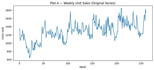
 week_index  trend_forecast  season_forecast  sales_forecast
0         261     1473.953221       379.560016     1853.513237
1         262     1474.612396       390.811184     1865.423580
2         263     1475.271570       -73.078943     1402.192627
3         264     1475.930744       113.327963     1589.258707
4         265     1476.589919        -2.495993     1474.093926
5         266     1477.249093       172.367070     1649.616164
6         267     1477.908268       -64.937843     1412.970425
7         268     1478.567442       -10.745014     1467.822428
8         269     1479.226617       100.006290     1579.232907
9 270 1479.885791 -12.914374 1466.971417This forecast is decision-useful because it makes assumptions visible. If the projected series rises, you can ask whether the rise is driven by trend continuation or seasonal repetition. That makes it easier to connect the forecast to staffing, inventory, and promotion timing.
If the remainder remains large or visibly patterned, the analyst may be forcing visible structure onto a series that still contains unresolved behavior. If the projected trend looks smooth but conflicts with business context, the problem is not the graph—it is the assumption of persistence.
Treating a smooth component as a certain component. Smoothness is a feature of estimation, not proof that the future will behave the same way.
Explicit structure helps NorthStar decide how to respond, not just whether to respond. Trend may justify more durable commitments; seasonality may justify temporary actions; remainder may justify caution.
Which component drives most of the 26-week forecast movement? Why does that matter for planning risk?
Now that you have practiced explicit visible-structure forecasting, the next step is to reason more carefully about when these assumptions are trustworthy—and when AI may help clarify the logic without making the decision for you.
Using AI as a learning partner to test explicit forecasting logic
This LearningLab reinforces the central idea of Chapter 4:
When we estimate trend and seasonality explicitly, we are not just describing data—we are imposing structure on how the future is expected to behave.
Using AI as both a learning partner and a thinking partner, this LearningLab helps you move from:
The objective is to:
This LearningLab reinforces:
AI is used not to build models, but to stress-test the structure you impose.
In the preceding SkillBox, you estimated trend and seasonality explicitly using methods such as:
These methods produce clean, interpretable components. However, this clarity comes with a hidden commitment:
You are assuming that the structure you estimated will continue into the future.
This LearningLab focuses on evaluating that assumption.
AI is used here to:
Key principle:
Explicit structure improves clarity—but can reduce flexibility.
NorthStar analysts have now moved beyond decomposition. They are actively estimating structure:
This creates new decision risks:
Managers begin asking:
To support these questions, analysts use AI to:
AI does not decide which structure is correct—it helps reveal what each structure implies.
You will engage with AI in three structured modes:
Reinforce → Extend → Explore
Work through them in order.
Build a clear understanding of explicit structural modeling.
“Key concepts from Chapter 4.
“I understand how trend and seasonality are explicitly modeled and what assumptions are involved.”
Evaluate how different structural choices affect forecasts.
Optionally explore additional analytical concepts or methods that interest you but not covered in the chapter.
“I can evaluate and compare structural modeling choices and understand their consequences.”
Connect structural modeling choices to real-world decisions and risks.
“I understand how structural assumptions affect decisions and when they may fail.”
After completing all three modes:
The goal is to interrogate structure—not accept it blindly.
Prepare a structured response including:
Explain how trend and seasonality were modeled and what assumptions were made.
Identify one structural assumption that could fail and describe its impact on forecasts.
You must:
Principle:
AI can suggest structures—but cannot validate their appropriateness.
Explicit structural models convert patterns into equations:
This enables:
But introduces risk:
AI can:
But cannot:
Insight:
Explicit structure improves clarity—but must always be questioned.
You have now moved from:
interpreting structure → imposing structure
The next step is:
imposing structure → designing how it supports decisions
How should structural models be used in:
The DesignStudio will move from:
model specification → structural judgment → decision integration
This DesignStudio develops decision design capability. Students use the explicit-structure forecast not to tune a model, but to design a planning response that reflects the forecast’s visible components.
NorthStar RetailGroup is preparing its next 26-week operating cycle. The explicit forecast shows mild upward trend growth along with strong recurring seasonal peaks.
Leadership must decide how much of the projected increase should drive durable commitments and how much should be treated as temporary recurring movement.
A permanent response to temporary seasonality creates overcommitment. A temporary response to durable trend creates underpreparation and lost service quality.
Respond to the following prompts:
A one-page planning note that distinguishes durable action, temporary action, and caution zones.
Strong responses will connect component interpretation to operational action, acknowledge uncertainty, and avoid treating the forecast as a single unquestioned number.
Explicit forecasting is most useful when it helps the organization respond differently to different kinds of projected movement.
How does separating visible structure improve organizational accountability?
NorthStar helps us design action in a familiar context. The next step is to transfer that reasoning to a new setting where visible structure matters but the stakes are different.
A regional electric utility is preparing demand forecasts for next year’s capacity planning cycle. Historical demand shows a long-run directional shift associated with population movement and efficiency programs, along with strong seasonal weather-related cycles. Leaders want a forecast that is explainable, auditable, and suitable for regulatory discussion.
The analytics team proposes an explicit-structure forecast that separates trend and seasonality before projecting them forward. The result is easy to explain: one part reflects long-term movement, one part reflects recurring seasonal rhythm, and the remainder is treated as uncertainty.
The forecast appears reasonable. But some team members worry that visible component forecasting may not be enough if recent changes reflect deeper forms of temporal dependence not captured by trend and seasonality alone.
Should leadership rely on the explicit visible-structure forecast for capacity planning, or should it treat the forecast as useful but incomplete?
Write a short recommendation that answers:
A concise executive recommendation.
What does this case reveal about the difference between interpretability and completeness?
A forecast can be highly explainable and still leave important dependence unresolved. Good decision design recognizes both the value and the boundary of visible structure.
Visible temporal structure improves forecasting not because it guarantees correctness, but because it makes assumptions about persistence and repetition explicit. When trend and seasonality are separated, forecast behavior becomes easier to interpret, communicate, and challenge. Yet visible structure is only part of temporal behavior, which means transparency must eventually be paired with deeper forms of validation.
At NorthStar RetailGroup, the forecasting system has now moved beyond signal extraction into visible structural representation. The organization can distinguish which projected movement appears tied to longer-term trend and which appears tied to recurring seasonal rhythm, allowing staffing, replenishment, and promotional decisions to be aligned more deliberately. This improves cross-functional accountability because finance, operations, and merchandising can now discuss the same forecast through a shared structural language. At the same time, NorthStar has reached an important limit: not all temporal dependence is visible, and some risks remain hidden beneath apparently sensible components.
Explain reasoning clearly. Distinguish signal from noise. Connect analysis to decisions. Avoid purely technical answers.
When forecast movement comes from trend, organizations may justify more durable commitments; when it comes from seasonality, they should often prefer temporary and flexible responses.
A common mistake is to assume that a smooth estimated trend is automatically trustworthy simply because it looks stable on a chart.
This chapter showed how forecasts become more interpretable when visible temporal structure is separated into trend and seasonality. But some forms of time behavior do not present themselves as visible components at all. A forecast may appear structurally sensible and still miss how the series depends on its own recent history. Chapter 5 begins there: with hidden temporal structure, where memory, dependence, and unseen persistence must be modeled even when they cannot be cleanly displayed.

