Designing Hidden Temporal Structure in Forecasting:
Dependence, Memory, and Implicit Time Behavior
In many organizations, the most dangerous forecasting mistake is not failing to see visible structure. It is assuming that what cannot be seen does not matter.
A sales series may show no obvious trend break. A demand curve may look seasonally familiar. A smoothed forecast may appear calm and reasonable. Yet underneath that visible surface, the series may still carry memory: recent shocks may linger, past values may continue to shape current outcomes, and short-term disturbances may echo forward in ways that are not immediately visible on a chart.
This chapter begins where Chapter 4 deliberately stopped. Visible structure—trend and seasonality—helps analysts explain what a forecast appears to contain. But visible structure does not fully explain how a series behaves over time. Some temporal behavior is hidden in dependence itself: in the way observations remember the past, absorb shocks, and gradually return to stability. When forecasts are used for capacity, risk, replenishment, or operational control, that hidden structure matters.
Forecasting by design therefore requires a second structural question. After separating what can be seen, how should we represent what the series remembers?
In earlier chapters, the book developed a progression from seeing patterns to representing them. Chapter 2 introduced smoothing as a way to reduce noise and support fast decision sensemaking. Chapter 3 used decomposition to separate trend, seasonality, and irregular variation so that temporal structure could be interpreted more clearly. Chapter 4 extended that logic into forecasting by showing how visible structure can be projected explicitly through trend and seasonal components.
This chapter addresses a limitation left unresolved at the end of Chapter 4. Not all time structure is visible. Even after trend and seasonality are recognized, forecasts may still fail because the series carries hidden dependence: recent observations may influence future values, shocks may persist, and short-run movements may contain systematic temporal memory rather than mere noise.
The focus now shifts from visible structure to hidden structure. Instead of asking, “What components can we separate and project?” this chapter asks, “How does the series depend on its own past once visible structure has been stabilized?” That question leads to the logic of implicit-structure forecasting, represented in this chapter through ARIMA and seasonal ARIMA as foundational methods for handling dependence, memory, and shock correction.
The goal is not to turn forecasting into a technical contest. The goal is to help students understand how hidden temporal structure changes what a forecast assumes, how it should be validated, and why some decision settings value disciplined dependence more than visible explanation. In other words, this chapter extends the forecasting-by-design philosophy from component visibility to behavioral discipline.
This chapter follows the Forecast-by-Design reasoning progression:
Observe → Understand → Practice → Reason → Design → Decide → Integrate → Consolidate → Continue
After completing this chapter, students should be able to:
When visible structure is not enough, how should forecasting systems represent what the past still remembers?
When an electric utility forecasts demand, the problem is not only how much power customers will need. The deeper problem is how the system remembers.
At Tokyo Electric Power Company (TEPCO), demand forecasting supports decisions that carry operational, financial, and regulatory consequences. Maintenance schedules, reserve commitments, fuel arrangements, and grid reliability plans all depend on the forecast. A mistake is not merely an inaccurate number. It can become a capacity shortfall, an unnecessary reserve purchase, or a regulatory question about whether the planning process was disciplined enough to justify the decision.
For years, TEPCO’s analysts had strong ways to see visible structure. Seasonal peaks were familiar. Summer heat raised cooling demand. Winter cold affected regional loads differently. Longer-term shifts in efficiency and industrial activity altered the broad direction of the series. These patterns could be plotted, discussed, and explained. In a planning meeting, people could point to the chart and say, “There is the trend,” or “There is the seasonal cycle.”
But over time, the forecasts began to reveal a harder problem. Even after visible structure was acknowledged, the series still behaved in ways that were not easy to explain component by component. A heatwave did not disappear when the week ended; its effect lingered. A demand shock in one period influenced subsequent periods unevenly. Small deviations accumulated. Some short-run changes faded quickly, while others persisted just long enough to distort planning if treated as noise.
The issue was no longer whether the analysts could see structure. The issue was whether they could represent memory.
The forecasting team realized that decomposition and explicit projection helped answer one type of managerial question: What parts of this forecast reflect trend and seasonality? But another question had become just as important: How does current demand depend on what happened recently, and how long do shocks continue to matter? That question could not be answered by simply displaying components more clearly.
The team turned to ARIMA-style forecasting not because they wanted a more complicated method, but because they needed a more disciplined way to encode time dependence. Instead of projecting visible components directly, the method stabilized the series, modeled how current values related to recent history, and checked whether unexplained structure still remained in the residuals. The forecast became less narratively transparent but more behaviorally accountable.
The change altered internal conversations. Managers stopped asking only, “What trend are we seeing?” and began asking, “Has the series been stabilized? Does the model still leave structure unexplained? Are we treating a temporary shock as if it will persist?” The forecast was no longer just a number supported by a chart. It became a claim about temporal memory that had to be defended.
This chapter focuses on forecasting environments like that one. In such settings, visible structure matters—but it is not enough. Hidden structure must also be handled responsibly. That is where implicit-structure forecasting begins.
Chapter 4 showed how forecasts can be designed by separating visible temporal structure into trend and seasonality, projecting those components, and recombining them. That approach is powerful when organizations need explanation, shared interpretation, and visible accountability. It helps people see what part of a forecast reflects long-run movement, what part reflects recurring cycles, and what part should be treated as uncertainty.
But visible structure is not the whole story.
A time series may retain important behavioral structure even after those visible elements are recognized. Recent values may influence current values. Shocks may echo into the future. Errors may cluster rather than disappear. Some series “forget” quickly. Others remember longer than managers expect. These features are not always visible in a decomposition chart, but they strongly affect how forecasts behave.
This is the unresolved problem left by explicit structure. A decomposition can show what the series appears to contain. It does not fully specify how the series moves from one period to the next.
That is why this chapter shifts attention from visible structure to hidden structure. Hidden structure refers to the temporal relationships embedded in the sequence itself: persistence, dependence, lagged influence, and shock correction. In forecasting terms, it asks whether the past continues to shape the future even when visible components have already been accounted for.
A simple business analogy helps. Visible structure is like reading a company’s organizational chart. You can see departments, roles, and reporting lines. Hidden structure is like understanding how work actually flows through the organization: who influences whom, where delays accumulate, and how one disruption affects later decisions. Both matter, but they answer different questions. A good forecast design must know whether it needs a map of the visible pieces, a model of the underlying dependence, or both.
This chapter therefore introduces the logic of implicit structure: rather than forecasting visible components separately, the analyst stabilizes the series and models how it depends on its own past. That design choice sacrifices some transparency but strengthens behavioral discipline.
Analytical Framing: Structure → Behavior → Trust
In this chapter, structure is no longer just what can be seen in components. It also includes the hidden dependence that governs behavior over time. Trust therefore depends less on visual plausibility and more on whether the modeled behavior leaves no meaningful structure behind.
If analysts ignore hidden structure, organizations may treat temporary shocks as permanent change, underestimate persistence, or overreact to short-term disturbances. In staffing, replenishment, energy planning, or risk management, those mistakes can create costly commitments.
A common misinterpretation is to assume that once trend and seasonality are recognized, the remaining variation is merely random noise. In many real settings, the remainder still carries memory. Treating hidden dependence as noise can produce forecasts that look reasonable but behave unreliably.
Suppose NorthStar RetailGroup tracks weekly unit sales for an everyday essentials category. The visible seasonal cycle is clear: some weeks rise predictably due to calendar effects. Yet even after seasonal timing is understood, unexpected stockouts, promotions, or local disruptions may influence several subsequent weeks. The series is not only seasonal; it is dependent.
To work with hidden structure responsibly, analysts need a language for dependence, memory, and stabilization. The next section introduces that language.
When analysts say that a time series has dependence, they mean that current values are not independent snapshots. What happened recently still influences what happens now. This influence may be strong or weak, short-lived or persistent, orderly or irregular. Forecasting hidden structure begins by taking that dependence seriously.
Three plain-language ideas are especially useful.
First, memory.
Some series remember the past for only a short time. A one-week demand spike may disappear almost immediately. Other series carry the effect longer. A disruption in supply, a pricing change, or a demand surge may continue to shape behavior across several future periods. Memory does not necessarily appear as visible trend or seasonality. It appears as temporal carryover.
Second, persistence.
Persistence asks how strongly the current level depends on recent levels. If recent observations strongly influence the present, the series has more persistence. If new values quickly detach from recent history, persistence is weaker. In forecasting, persistence affects how quickly a model should respond and how much recent history should matter.
Third, shock correction.
A shock is a disturbance that pulls the series away from its expected path. Some shocks dissipate quickly. Others echo through later periods. Hidden structure includes not just whether shocks happen, but how the series absorbs and corrects them over time.
These ideas help explain why forecasts built on the same data can behave differently. One method may separate visible components and treat the remainder as uncertainty. Another may encode how the series remembers its past and corrects recent disturbances. Neither is automatically better. Each is a different design choice about what temporal structure deserves formal representation.
A practical contrast clarifies the distinction:
This chapter does not treat these questions as rivals. It treats them as different forecasting philosophies.
Let Yₜ denote the observed series. Visible-structure methods often emphasize decompositions such as trend plus seasonality plus remainder. Hidden-structure methods instead focus on how Yₜ relates to earlier values such as ( Yₜ -1 , Yₜ -2 ), and earlier shocks ( εₜ -1 , εₜ -2 ). The mathematics can be formalized later, but the conceptual point is already clear: one design makes structure visible; the other embeds structure in temporal dependence.
For a manager, dependence means that a recent disturbance may not be over just because the calendar moved forward. The past still matters operationally. A promotion week may affect the next week’s demand. A stockout may distort several later observations. A weather shock may not vanish immediately. Forecasts that ignore such dependence can look clean but mislead decisions.
Visible structure answers “What shape do we see?” Hidden structure answers “How does that shape keep moving?” Both are legitimate, but confusing one for the other leads to poor forecast design.
Another common mistake is to use the word “noise” too quickly. If residual movement still follows a temporal pattern, it is not yet just noise. The analyst may still be looking at dependence that the current forecast design has failed to represent.
In a retail replenishment system, underestimating memory can lead to repeated overcorrections. In a utility setting, underestimating shock persistence can distort reserve planning. In both cases, the cost comes not from bad arithmetic, but from a poor representation of temporal behavior.
NorthStar sees an unusual sales surge during a regional weather event. The week after the surge drops, but not back to normal. Two more weeks remain elevated as customers restock unevenly. A visible seasonal explanation is not enough. The series is showing memory.
To model hidden structure, analysts need a way to separate persistent dependence from unstable visible movement. That is why stabilization comes next.
Implicit-structure forecasting does not begin by modeling the series exactly as observed. It begins by asking whether the series is stable enough for dependence to be interpreted meaningfully.
If a time series is still drifting strongly upward, or if strong seasonal swings dominate the pattern, then short-run dependence can be difficult to interpret cleanly. The visible movement may overwhelm the hidden relationships. In those situations, the series is often stabilized first so that its dependence can be modeled more responsibly.
This is the role of differencing in ARIMA-style forecasting.
Differencing does not try to “discover” trend or seasonality as visible components. Instead, it reduces their dominating effect so that the series fluctuates around a more stable level. Once that stabilization is achieved, the analyst can ask a more disciplined question: after visible drift has been reduced, how does the series still depend on its past?
A simple analogy helps. Suppose a business wants to study the steering behavior of a vehicle. If the car is still driving up a steep hill and hitting recurring road bumps, it is harder to isolate the steering pattern itself. Stabilization is like moving the vehicle to a flatter test environment so the steering behavior becomes easier to observe.
This is why ARIMA’s logic begins with transformation before dependence. The method assumes that hidden structure becomes easier to represent once dominant visible movement has been absorbed or removed.
With first differencing, the analyst studies changes from one period to the next:
This helps reduce long-run drift.
With seasonal differencing of season length s, the analyst compares a period to its seasonal counterpart:
This helps reduce recurring seasonal influence.
Combined differencing applies both ideas, d times and D times respectively, when needed:
Students do not need to memorize the notation. The important idea is design logic: stabilization makes hidden dependence easier to interpret.
After stabilization, the series should behave more like a sequence fluctuating around a relatively constant level rather than trending or cycling visibly. That does not mean all uncertainty is gone. It means the analyst has created a better setting for modeling persistence and shock correction.
If stabilization is skipped when needed, the model may confuse visible drift with true dependence. If stabilization is overused, the analyst may strip away meaningful long-term signal. Either mistake can undermine trust.
A frequent error is to treat differencing as a technical ritual rather than an interpretive decision. Over-differencing can create artificial instability. Under-differencing can leave visible structure that distorts hidden dependence. The question is not “Did we difference?” but “Did stabilization improve behavioral interpretability?”
This is where Structure → Behavior → Trust becomes especially important. Stabilization is not done for elegance. It is done so that the series’ behavior can be modeled in a way that earns trust.
NorthStar’s weekly essentials sales show both a slow upward drift and recurring annual seasonality. If analysts want to study how one unusual week affects subsequent weeks, they may first reduce the visible drift and seasonality so that the remaining dependence is easier to model.
Once the series has been stabilized, implicit forecasting can encode persistence and shock correction directly. That is the role of ARIMA and SARIMA.
ARIMA stands for AutoRegressive Integrated Moving Average. Its seasonal extension, SARIMA, adds seasonal dependence to the same basic logic. In this chapter, ARIMA/SARIMA serves as the representative method for hidden temporal structure.
The key design idea is simple: instead of projecting visible components separately, ARIMA models how the stabilized series depends on its own past and on past shocks.
This logic can be understood through three connected roles.
The integrated component refers to differencing. It helps reduce dominating trend or seasonality so that the remaining series is more stable and suitable for dependence modeling.
The autoregressive component captures how strongly current behavior depends on recent past values:
where i, i=1,2,… are estimated coefficients based on observed data.
This component captures persistence: how strongly current values depend on recent past values.
The moving-average component captures how recent disturbances or errors continue to affect subsequent observations:
where i, i=1,2,… are estimated coefficients based on observed data.
This reflects the system’s correction behavior.
A compact expression sometimes used to represent a complete ARIMA design is:
where
represents unpredictable residuals — what remains after systematic structure and dependence have been accounted for.
Students do not need to work through the formula mechanically. Read it as a structural summary: the series is first stabilized, then modeled through dependence and shock correction, leaving a residual innovation term that ideally contains no remaining structure.
Once temporal dependence has been estimated, ARIMA produces forecasts directly from the learned relationships :
This expression is schematic rather than computational. It indicates that forecasts are generated directly from past observations through learned temporal dependence, without projecting and recombining visible components.
With ARIMA, what you gain is discipline and stability; what you give up is visibility into individual structural components.
Unlike STL, ARIMA does not produce separate forecasted trend and seasonality curves for inspection. It forecasts the series directly from learned temporal relationships. What becomes visible is not the components, but the model’s behavioral discipline.
ARIMA is valuable when the organization cares deeply about whether the forecasting process has captured dependence responsibly. It is especially useful when consistency, auditability, and residual-based validation matter more than component-level storytelling.
STL says, in effect, “Let us show the forecast’s visible pieces.”
ARIMA says, in effect, “Let us stabilize the series and model how it behaves over time.”
That difference is philosophical, not merely technical.
If a forecast is used to trigger replenishment orders, set reserve thresholds, or support monthly risk reporting, hidden dependence may matter more than visible explanation. In those settings, a model that reacts with disciplined memory can be more useful than one that is easier to narrate.
A serious mistake is to believe that once ARIMA produces a forecast, the job is done. In implicit-structure forecasting, producing a forecast is not the same as justifying it. Because the structure is less visible, validation becomes the primary safeguard.
Models don’t decide—systems do.
An ARIMA forecast may be statistically disciplined, but human decision-makers must still judge whether that discipline fits the organization’s context, communication needs, and risk tolerance.
NorthStar may use ARIMA-style forecasting when weekly demand shows persistent carryover from promotions, stockouts, or local disruptions that are not well handled by visible component projection alone. The benefit is not prettier charts. The benefit is a more disciplined representation of memory.
The SkillBox later in the chapter will make this workflow concrete using NorthStar’s weekly sales series. Before that, the final conceptual section compares explicit and implicit structure directly so students can understand the design trade-off.
By this point, the chapter has established that forecasting can represent time in at least two foundational ways.
The explicit path separates visible structure into components such as trend and seasonality, then projects them forward.
The implicit path stabilizes the series and models how it depends on its past.
The choice is not about which method is more modern, more advanced, or automatically more accurate. It is about which design better fits the decision environment.
|
Dimension |
Explicit Structure (STL-style logic) |
Implicit Structure (ARIMA/SARIMA logic) |
|---|---|---|
|
What structure looks like |
Visible components |
Hidden dependence |
|
Main question |
What visible patterns persist? |
What does the series remember? |
|
Forecasting logic |
Separate, project, recombine |
Stabilize, encode dependence, forecast directly |
|
Main evidence of quality |
Component plausibility |
Residual discipline |
|
Communication strength |
Easier to explain |
Harder to explain |
|
Validation strength |
Assumptions can be inspected |
Behavior can be tested statistically |
|
Primary risk |
Mis-projecting unstable components |
Hiding structural misspecification behind technical form |
|
Best decision fit |
Shared planning and explainability |
Consistency, auditability, and disciplined control |
This comparison highlights a central forecasting-by-design principle: the important choice is not merely the algorithm. It is the representational contract the organization is willing to accept.
An explicit-structure forecast tells stakeholders, “Here is the trend we believe in; here is the seasonal cycle we expect to continue.”
An implicit-structure forecast tells them, “Here is how the series behaves after stabilization, and here is the evidence that no important dependence remains unmodeled.”
Both statements can support decisions. But they support different kinds of trust.
If leadership must explain the forecast to nontechnical partners, visible structure may be essential. If the forecast must pass methodological review and repeated monitoring, implicit discipline may be more important.
The wrong comparison is to ask only which method “wins.” The better comparison is to ask which method fails in a way the organization can tolerate. An explainable model may fail by oversimplifying dependence. A disciplined hidden-structure model may fail by being harder to communicate when major decisions require shared understanding.
NorthStar might use explicit structure for annual budgeting conversations where cross-functional explanation matters, but implicit structure for automated replenishment rules where disciplined response to short-run dependence matters more than narrative clarity.
The remainder of the chapter moves from concept to application. First, you will practice implicit-structure forecasting directly in the SkillBox. Then you will reason through its assumptions with AI, design decision processes around it, and decide when it should or should not be used.
From stabilized series to a defensible forecast
This SkillBox develops hands-on skill in forecasting with hidden temporal structure using ARIMA/SARIMA. The purpose is not to optimize parameters or compete for the best numerical fit. The purpose is to experience how implicit-structure forecasting stabilizes a series, encodes dependence, and requires validation when structure is no longer made visible through separate components.
NorthStar RetailGroup monitors weekly unit sales for an everyday essentials product line. The planning issue is not only whether sales rise or fall, but whether recent shocks and short-run movements continue to affect subsequent weeks. Forecasts are used to inform replenishment and operating decisions, so dependence must be handled responsibly.
Primary dataset: essentials_sales_lite.csv
This is the same NorthStar dataset used in earlier chapters so that changes in forecasting behavior can be traced to design choices rather than changing data context.
If hidden dependence is ignored, NorthStar may misread short-term carryover effects and issue replenishment decisions that either overreact or respond too slowly. In a high-volume essentials category, those errors can create stock pressure, working-capital distortion, or unstable service levels.
You will:
Python
# SkillBox 5 (Python): ARIMA/SARIMA implicit-structure forecasting
# Focus: stabilize -> encode dependence -> forecast -> validate
import pandas as pd
import numpy as np
import matplotlib.pyplot as plt
from statsmodels.tsa.statespace.sarimax import SARIMAX
from statsmodels.graphics.tsaplots import plot_acf
from statsmodels.stats.diagnostic import acorr_ljungbox
# 1) Load primary dataset
df = pd.read_csv("essentials_sales_lite.csv")
time_col = "week_index" if "week_index" in df.columns else None
x = df[time_col] if time_col else np.arange(1, len(df) + 1)
y = df["sales"].astype(float)
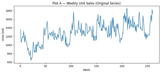
# Plot A — Original series
plt.figure(figsize=(10, 4))
plt.plot(x, y)
plt.title("Plot A — Weekly Unit Sales (Original Series)")
plt.xlabel("Week")
plt.ylabel("Units Sold")
plt.show()
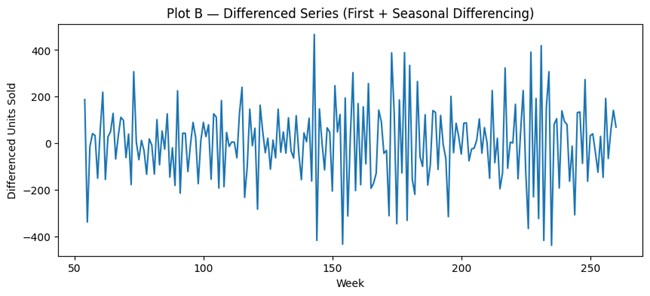
# 2) Stabilize: first + seasonal differencing (illustrative)
s = 52
y_diff_both = y.diff(1).diff(s)
plt.figure(figsize=(10, 4))
plt.plot(x, y_diff_both)
plt.title("Plot B — Differenced Series (First + Seasonal Differencing)")
plt.xlabel("Week")
plt.ylabel("Differenced Units Sold")
plt.show()
# 3) Fit a bounded, explainable SARIMA baseline
order = (1, 1, 1)
seasonal_order = (1, 1, 1, s)
model = SARIMAX(
y,
order=order,
seasonal_order=seasonal_order,
enforce_stationarity=False,
enforce_invertibility=False
)
res = model.fit(disp=False)
print(res.summary())
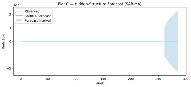
# 4) Forecast
H = 26
pred = res.get_forecast(steps=H)
yhat = pred.predicted_mean
ci = pred.conf_int()
last_week = int(x.iloc[-1]) if time_col else len(df)
future_x = np.arange(last_week + 1, last_week + H + 1)
plt.figure(figsize=(10, 4))
plt.plot(x, y, label="Observed")
plt.plot(future_x, yhat, label="SARIMA Forecast")
plt.fill_between(future_x, ci.iloc[:, 0], ci.iloc[:, 1], alpha=0.2, label="Forecast interval")
plt.title("Plot C — Hidden-Structure Forecast (SARIMA)")
plt.xlabel("Week")
plt.ylabel("Units Sold")
plt.legend()
plt.show()
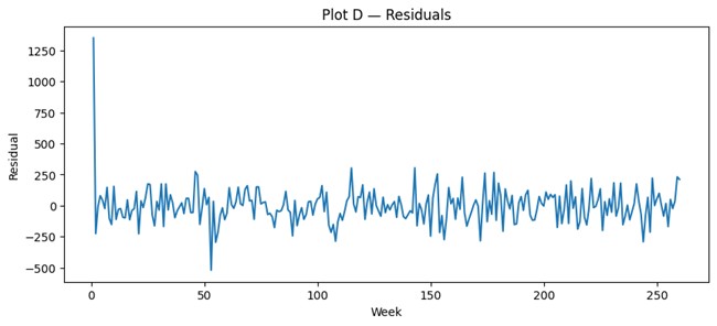
# 5) Residual validation
resid = res.resid
plt.figure(figsize=(10, 4))
plt.plot(x, resid)
plt.title("Plot D — Residuals")
plt.xlabel("Week")
plt.ylabel("Residual")
plt.show()
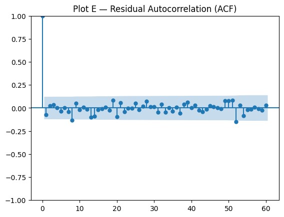
plt.figure(figsize=(8, 3))
plot_acf(resid.dropna(), lags=60)
plt.title("Plot E — Residual Autocorrelation (ACF)")
plt.show()
lb = acorr_ljungbox(resid.dropna(), lags=[12, 26, 52], return_df=True)
print("\nLjung–Box test:")
print(lb)
# 6) Compact forecast table
out = pd.DataFrame({
"week_index": future_x,
"sales_forecast": yhat.values,
"lower": ci.iloc[:, 0].values,
"upper": ci.iloc[:, 1].values
})
print(out.head(10))R
# SkillBox 5 (R): ARIMA/SARIMA implicit-structure forecasting
# Focus: stabilize -> encode dependence -> forecast -> validate

df <- read.csv("essentials_sales_lite.csv", stringsAsFactors = FALSE)
x <- if ("week_index" %in% names(df)) df$week_index else 1:nrow(df)
y <- as.numeric(df$sales)

# Plot A — Original series
plot(x, y, type="l",
     main="Plot A — Weekly Unit Sales (Original Series)",
     xlab="Week", ylab="Units Sold")

# 2) Differencing
s <- 52
y_diff_both <- diff(diff(y, lag=1), lag=s)

plot(x[(s+2):length(x)], y_diff_both, type="l",
     main="Plot B — Differenced Series (First + Seasonal Differencing)",
     xlab="Week", ylab="Differenced Units Sold")

# 3) Fit bounded baseline SARIMA
y_ts <- ts(y, frequency = s)
fit <- arima(y_ts,
             order = c(1,1,1),
             seasonal = list(order = c(1,1,1), period = s),
             include.mean = FALSE,
             method = "CSS")

fit

# 4) Forecast
H <- 26
fc <- predict(fit, n.ahead = H)

z <- qnorm(0.975)
lower <- fc$pred - z * fc$se
upper <- fc$pred + z * fc$se
future_x <- (max(x) + 1):(max(x) + H)

plot(x, y, type="l",
     main="Plot C — Hidden-Structure Forecast (SARIMA)",
     xlab="Week", ylab="Units Sold")
lines(future_x, fc$pred, lty=2)
lines(future_x, lower, lty=3)
lines(future_x, upper, lty=3)
legend("topleft",
       legend=c("Observed", "Forecast", "Approx. interval"),
       lty=c(1,2,3), bty="n")

# 5) Residual checks
resid <- residuals(fit)

plot(x, c(rep(NA, length(x)-length(resid)), resid), type="l",
     main="Plot D — Residuals",
     xlab="Week", ylab="Residual")

acf(resid, main="Plot E — Residual Autocorrelation (ACF)")

Box.test(resid, lag=12, type="Ljung-Box")
Box.test(resid, lag=26, type="Ljung-Box")
Box.test(resid, lag=52, type="Ljung-Box")

# 6) Compact forecast table
out <- data.frame(
  week_index = future_x,
  sales_forecast = as.numeric(fc$pred),
  lower = as.numeric(lower),
  upper = as.numeric(upper)
)

head(out, 10)
Key Outputs
                                     SARIMAX Results
=============================================================================
Dep. Variable:                              sales   No. Observations:                  260
Model:             SARIMAX(1, 1, 1)x(1, 1, 1, 52)   Log Likelihood               -2523.360
Date:                            Sat, 21 Mar 2026   AIC                           5056.719
Time:                                    00:48:06   BIC                           5071.871
Sample:                                         0   HQIC                          5062.874
                                            - 260
Covariance Type:                              opg
=============================================================================
                 coef    std err          z      P>|z|      [0.025      0.975]
------------------------------------------------------------------------------
ar.L1         -0.1439         -0        inf      0.000      -0.144      -0.144
ma.L1         -0.5963         -0        inf      0.000      -0.596      -0.596
ar.S.L52      -0.5705   1.48e-29  -3.86e+28      0.000      -0.570      -0.570
ma.S.L52   -1.976e+13   1.47e-32  -1.34e+45      0.000   -1.98e+13   -1.98e+13
sigma2      8.619e-14   1.53e-10      0.001      1.000   -3.01e-10    3.01e-10
=============================================================================
Ljung-Box (L1) (Q):                   1.44   Jarque-Bera (JB):                 0.50
Prob(Q):                              0.23   Prob(JB):                         0.78
Heteroskedasticity (H):               0.98   Skew:                             0.13
Prob(H) (two-sided):                  0.94   Kurtosis:                         2.87
=============================================================================

Warnings:
[1] Covariance matrix calculated using the outer product of gradients (complex-step).
[2] Covariance matrix is singular or near-singular, with condition number    inf. Standard errors may be unstable.
Ljung–Box test:
      lb_stat  lb_pvalue
12   8.053384   0.780945
26  20.361649   0.774116
52  41.914820   0.840057
   week_index  sales_forecast         lower         upper
0         261     1886.361089 -1.136862e+07  1.137239e+07
1         262     1912.840317 -1.174617e+07  1.175000e+07
2         263     1503.243993 -1.246312e+07  1.246613e+07
3         264     1645.707171 -1.308635e+07  1.308964e+07
4         265     1556.571739 -1.368876e+07  1.369187e+07
5         266     1714.599577 -1.426451e+07  1.426794e+07
6         267     1544.414741 -1.481836e+07  1.482145e+07
7         268     1690.437825 -1.535193e+07  1.535531e+07
8         269     1648.169039 -1.586775e+07  1.587104e+07
9         270     1566.782127 -1.636736e+07  1.637049e+07
An implicit-structure forecast becomes trustworthy not because it shows visible components, but because it behaves as though no important dependence has been left behind. Once the series is stabilized, the forecast reflects how the model believes the past continues to influence the future. Residuals therefore matter. If they still show structure, then the model may look disciplined without actually capturing the series responsibly.
Treating differencing and model fitting as automatic steps rather than judgment calls. A model can produce a forecast even when stabilization is poorly chosen or dependence remains unmodeled. Forecast production is not proof of forecast adequacy.
Implicit structure is often useful when the organization cares more about disciplined behavioral capture than about visible storytelling. It supports a defensible process: stabilize the series, encode dependence, and test whether meaningful structure remains. That logic can be especially valuable when forecasts feed repeated operational decisions.
The SkillBox showed how hidden structure can be modeled. The next component uses AI as a learning partner to reason more carefully about why stabilization and residual validation matter.
Using AI as a Learning and Thinking Partner
This LearningLab reinforces the central idea of Chapter 5:
In implicit structure models, patterns are not separated and specified—they are encoded through dependence and memory.
Instead of modeling trend and seasonality directly, models such as ARIMA represent structure through:
The objective is to:
This LearningLab reinforces:
AI is used not to build models, but to make invisible structure visible through reasoning.
In the preceding SkillBox, you implemented models that do not explicitly separate components, but instead:
These models are powerful because they adapt to complex patterns. However, they also introduce a critical challenge:
The structure is no longer directly observable—it must be inferred.
This LearningLab focuses on understanding and evaluating that implicit structure.
AI is used here to:
Key principle:
Implicit structure increases flexibility—but reduces transparency.
NorthStar analysts have moved from explicit decomposition to dependence-based modeling.
Instead of projecting trend and seasonality directly, they now rely on:
This introduces new questions:
Managers no longer see clear components—they see outputs that depend on hidden structure.
To support interpretation, analysts use AI to:
AI does not reveal the true structure—it helps reason about what the model is doing.
You will engage with AI in three structured modes:
Reinforce → Extend → Explore
Work through them in order.
Understand dependence, memory, and implicit structure.
“The key concepts from Chapter 5.
“I understand how dependence and memory define implicit structure.”
Interpret and evaluate implicit structure in models.
Optionally explore additional analytical concepts or methods that interest you but not covered in the chapter.
“I can interpret implicit structure and assess whether it makes sense.”
Connect implicit structure to decision reliability and system behavior.
“I understand how implicit structure affects decisions and how to monitor it.”
After completing all three modes:
The goal is to understand the model—not just run it.
Prepare a structured response including:
Explain how your model represents dependence and memory.
Assess whether residual behavior supports the model assumptions.
You must:
Principle:
AI can describe models—but cannot validate their correctness.
Implicit structure models encode patterns through dependence:
Unlike explicit models:
Validation depends on diagnostics:
AI can:
But cannot:
Insight:
Implicit structure is powerful—but must be justified through diagnostics.
You have now moved from:
The next step is:
How do we evaluate whether these structures can be trusted over time?
The DesignStudio will move from:
model interpretation → diagnostic evaluation → decision reliability
This DesignStudio develops decision design capability by asking students to build a governance response around implicit-structure forecasting. The focus is not on parameter selection. It is on how an organization should communicate, defend, monitor, and act on a forecast whose logic is grounded in temporal dependence rather than visible components.
NorthStar RetailGroup is considering an implicit-structure forecasting process for a high-volume essentials category. Recent weeks have shown carryover effects from promotions, supply interruptions, and short-lived stockouts. Senior operations leaders are willing to accept a less visually intuitive forecast if it produces more disciplined planning behavior. Finance, however, wants a process that can be explained and reviewed consistently.
NorthStar must decide how to govern an ARIMA/SARIMA-based forecasting process for replenishment and short-horizon planning. The issue is not whether the model can produce forecasts. The issue is how the organization will justify their use, communicate their meaning, and define when the forecasts should be trusted or challenged.
Respond to the following prompts:
Prepare a short decision memo that:
Strong responses will:
Hidden structure often requires stronger process design around the model because the method itself is less narratively transparent. When assumptions are less visible, governance must become more explicit.
Which creates greater organizational risk in your judgment: a forecast that is easy to explain but weaker in hidden dependence, or a forecast that is behaviorally disciplined but harder to communicate? Why?
The DesignStudio asks how a single organization should govern hidden-structure forecasting. The Mini-Case now asks you to choose between forecasting paths in a different high-stakes context.
A regional electric utility is preparing next-year demand forecasts for capacity planning. Historical demand shows visible seasonality tied to weather and usage cycles, but it also shows short-run dependence: heatwaves affect not only the week in which they occur, but several subsequent weeks. Unexpected outages, industrial shifts, and abnormal temperature patterns appear to leave temporary but meaningful carryover effects.
The analytics team presents two forecasting options using the same historical data.
Senior leadership values transparency because the forecast must be explained to regulators and the board. At the same time, the forecast will also guide operational planning, where disciplined response to short-run dependence matters.
No accuracy metrics are provided. Both forecasts appear plausible. Leadership wants a recommendation based on decision fit, accountability, and risk.
Which forecasting path should leadership prefer for this capacity planning context, and why? Your answer must address:
Write a recommendation that addresses the following:
A concise advisory memo to senior leadership.
If conditions become more volatile midyear, which part of your recommendation would you revisit first?
Forecasting choices become more difficult when organizations need both visible explanation and disciplined behavioral capture. In such settings, the right design question is not “Which model wins?” but “Which failure mode can the organization manage more responsibly?”
Visible structure shows what a forecast appears to contain, but hidden structure determines how the series continues to behave. ARIMA/SARIMA matters not because it is more technical, but because it formalizes dependence, memory, and shock correction after stabilization. Forecast-by-Design therefore requires analysts to ask not only what the future looks like, but what the past is still doing inside the forecast.
NorthStar RetailGroup now recognizes that some forecast behavior cannot be explained adequately through projected trend and seasonality alone. In the essentials category, recent promotions, stockouts, and local disruptions appear to create short-run carryover effects that require a hidden-structure lens. The analytics team therefore adds an implicit-structure workflow to its forecasting system, using stabilization, dependence modeling, and residual review for short-horizon operational planning. This does not replace visible-structure forecasting; it expands the organization’s forecasting discipline by matching method choice to decision use. NorthStar’s system is becoming more mature because it now sees forecasting not as one model, but as a set of designed representations of time.
Explain your reasoning clearly. Distinguish signal from noise. Connect analytical choices to decisions. Avoid purely technical answers that do not address interpretation, accountability, or organizational use.
Use hidden-structure forecasting when disciplined behavioral capture matters more than component-level storytelling, especially in repeated operational settings where short-run dependence shapes decisions.
Do not assume that once visible trend and seasonality are recognized, the remaining variation is merely noise. Some of it may still be meaningful dependence.
This chapter showed how hidden temporal structure can be represented through stabilization, dependence, and residual discipline. But a critical question remains unresolved: How do we know whether the forecasted behavior is trustworthy enough to support action over time? The next chapter addresses that problem directly by focusing on diagnostics, validation, forecast uncertainty, and the conditions under which forecasting systems earn or lose trust.

