Smoothing Signals for Decision Sensemaking
Designing Fast, Interpretable Signals for Decisions
When weekly demand rises and falls unpredictably, reacting to every movement can cause organizations to chase noise rather than respond to real change.
Forecasting systems often fail not because their numbers are useless, but because decision-makers cannot tell whether a recent jump or drop reflects a meaningful shift or ordinary fluctuation. In fast-moving environments, acting too quickly on noisy data can be just as costly as acting too slowly when demand truly changes.
Smoothing addresses this problem by turning volatile observations into signals that are easier to read. It does not promise certainty. It helps organizations see direction clearly enough to respond at the right pace.
In Chapter 1, we learned to see demand through time. We observed that time-ordered data often contain visible movement, short-term fluctuation, and uncertainty that can easily mislead decision-makers. Chapter 2 takes the next step: it asks how analysts can convert that noisy flow of observations into signals that managers can actually use.
This chapter introduces smoothing as a tool for decision sensemaking rather than precise prediction. When data are noisy and decisions must be made quickly, precise forecasts are often unavailable—or unnecessary. In many business settings, managers do not need an exact estimate of next week’s demand. They need a reliable directional signal that helps them decide whether conditions are rising, falling, or staying roughly stable.
Smoothing provides that signal by reducing short-term volatility in time-ordered data. A smoothed series does not eliminate uncertainty, but it helps decision-makers distinguish meaningful movement from random fluctuation. In that sense, smoothing is not merely a statistical technique. It is a design choice about how quickly an organization learns from new information.
Different smoothing methods encode different beliefs about memory. Some methods treat recent history evenly. Others place greater weight on the newest observations. These choices affect how fast a signal responds, how stable it appears, and how likely managers are to trust it. That is why smoothing belongs not only to analytics, but also to decision design.
This chapter plays an early role in the book’s global spine of Structure → Behavior → Trust → Decision. In this chapter, the focus is primarily on Structure: how noisy data can be transformed into interpretable signals. At the same time, the chapter begins preparing for Behavior by showing that different smoothing designs respond differently to new information. Those response patterns matter because models don’t decide—systems do.
Throughout the chapter, we return to NorthStar RetailGroup to see how analysts convert volatile weekly sales data into usable managerial guidance. The goal is not to predict perfectly. The goal is to design fast, interpretable signals that support timely action under uncertainty.
This chapter follows the Forecast-by-Design reasoning progression:
Observe → Understand → Practice → Reason → Design → Decide → Integrate → Consolidate → Continue
The chapter unfolds as a continuous reasoning system:
This learning flow matters because the chapter is not teaching isolated techniques. It is teaching how to move from noisy observations toward reliable organizational action.
After completing this chapter, you should be able to:
How can analysts extract reliable signals from noisy time-series data so that managers can respond to meaningful changes without overreacting to short-term fluctuation?
In March 2020, millions of people developed a new habit: refreshing dashboards. Each morning, they checked graphs of COVID-19 cases, hoping the latest curve would reveal where the pandemic was headed.
The numbers were real, but they were often hard to interpret. One day case counts surged. The next day they dropped sharply. News headlines amplified every spike and dip, while public officials struggled to decide whether the situation had truly changed. Were infections suddenly accelerating, or were the numbers reflecting delays, backlogs, and reporting gaps?
Public health analysts quickly realized that much of the volatility came from the reporting process rather than the disease process itself. Weekend effects, testing delays, and administrative timing created jagged daily counts that were technically correct but behaviorally misleading. To make the data more interpretable, analysts increasingly plotted seven-day moving averages. The point was not to eliminate uncertainty. The point was to reveal direction.
Those smoothed curves helped decision-makers see whether conditions were broadly rising, stabilizing, or falling. They did not predict the future precisely. They helped people understand the present well enough to act.
The same logic appears in ordinary business settings.
It is 9:00 p.m. in downtown Indianapolis. The Pacers have just won a home game, and crowds are spilling into nearby restaurants. At The Fork & Flame, manager Sara glances at her dashboard. Recent guest counts have been volatile: Thursday 92, Friday 110, Saturday 128. Tonight’s game adds another layer of uncertainty.
Sara does not need a perfect forecast. She needs a quick directional read—enough to decide whether to call in another server or close the kitchen early.
Her dashboard shows a rolling average of recent evenings, adjusted for game nights. The smoothed signal is rising. That is enough.
She picks up the phone.
“Mike, can you come in for an hour?”
A forecast accurate to the last customer would not have improved the decision. A clear directional signal prevented a staffing problem.
From pandemic dashboards to pizza crowds, the lesson is the same: when observations are volatile, smoothing turns noisy data into usable signals. It helps decision-makers see structure without pretending uncertainty has disappeared.
That raises the chapter’s central question: what kind of smoothing design produces a signal that is fast enough to be useful, but stable enough to be trusted?
At NorthStar Retail Group, analysts face a recurring managerial problem: weekly demand fluctuates enough that raw observations can be difficult to interpret, yet operations still require timely decisions. Inventory needs must be reviewed. Staffing plans must be adjusted. Promotions must be timed. Waiting for perfect clarity is not realistic.
Smoothing is designed for this kind of environment. Its purpose is to reduce short-term fluctuation so that the underlying signal becomes easier to see. A helpful analogy is looking at a mountain range through morning fog. The fog hides distracting detail while still revealing the overall shape of the landscape. In much the same way, smoothing filters out some short-term variation so analysts can focus on direction and movement.
This is why smoothing fits naturally into the chapter’s place in the Structure → Behavior → Trust → Decision spine. It begins by clarifying structure. What is the signal doing beneath the week-to-week noise? Yet even at this early stage, smoothing also previews behavior, because different smoothing methods react differently to new information. That means the method itself influences what decision-makers notice and when they notice it.
Smoothing is therefore best understood as a decision-support tool, not a claim of certainty. It does not eliminate randomness. It makes the data interpretable enough for action when time pressure prevents deeper modeling.
Suppose NorthStar’s operations team observes these weekly sales for Everyday Essentials™:
Is demand rising? Or are these values simply bouncing around within normal variation?
If managers react to each weekly increase or decrease, they risk adjusting inventory and staffing too often. If they ignore the pattern entirely, they may miss the early signs of a meaningful shift. Smoothing helps resolve this tension by creating a signal that summarizes recent movement rather than amplifying every short-term fluctuation.
The stakes are practical. A signal that reacts too quickly may trigger unnecessary replenishment, staffing changes, or promotional responses. A signal that reacts too slowly may delay response to real demand shifts. In other words, smoothing affects not just interpretation, but the speed and quality of organizational action.
A common misinterpretation is to treat a raw spike as proof of a structural change. Another is to treat a smooth line as proof that uncertainty has disappeared. Both are mistakes. Smoothing helps clarify signal; it does not erase ambiguity.
Organizations smooth data because they need signals that support timely action without encouraging panic. In that sense, smoothing is an early example of a central lesson in this book: models don’t decide—systems do.
To understand why different smoothing methods produce different signals, we next need a more formal way to think about memory and weighting.
A time series consists of observations ordered through time. Smoothing transforms those raw observations into a more stable estimate of recent movement.
A minimal descriptive representation is:
Here, f(.) is the observed value at time t, and S t is the smoothed signal. The function f(.) represents a weighting rule that determines how much influence current and past observations receive. This formula is descriptive rather than technical. Its purpose is to highlight the key design question: how should the past influence the present?
That question matters because smoothing is fundamentally about memory design. Some methods remember recent history evenly. Others place more weight on new observations and let older information fade gradually. The weighting scheme determines how responsive the signal will be, how stable it will appear, and how much short-term volatility it will filter out.
A Simple Moving Average (SME) applies equal weight to the most recent (n) observations:
This produces a stable signal because no single point dominates the window. But it may respond slowly when conditions change.
Financial analysts often examine 10-day or 30-day moving averages of stock prices to filter daily volatility.
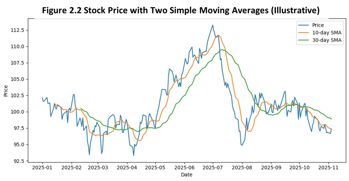
Flat memory protects managers from reacting too quickly.
A stable signal can look reassuring even when it is lagging behind a genuine turning point.
Simple Exponential Smoothing (SES) updates the signal by combining the newest observation with the previous smoothed value:
The parameter controls responsiveness. Larger values make the signal react more quickly to new information. Smaller values make it smoother and slower-moving.
Fading memory allows a signal to adapt more quickly when recent data matter more than older data.
High responsiveness can make routine noise look like meaningful change.
Methods such as LOESS (Locally Estimated Scatterplot Smoothing) assign greater weight to observations that are temporally close to the target point. This allows the smoothed curve to follow gradual nonlinear movement.
Rather than using a fixed window or a single decay rate, local smoothing assigns weights based on proximity in time: observations closer to the target point receive greater influence than those farther away.
These methods are especially useful for exploratory analysis and visualization because they can flexibly reveal underlying structure. However, they are often less transparent and harder to maintain in operational forecasting systems.
For this reason, LOESS appears in this chapter primarily as a visualization benchmark rather than a production signaling method.
Local smoothing can reveal shape and structure that simpler methods may miss.
Although visually appealing, local smoothers are often harder to explain, harder to maintain, and less transparent for routine operational decisions.
For that reason, LOESS appears in this chapter mainly as a visual benchmark, not as the primary operational signal.
Smoothing is strong at one thing: reducing short-term noise so that broad directional movement becomes easier to interpret. That is why it is so useful in dashboards, weekly reviews, and operational monitoring.
Its limitations are equally important. Smoothing does not explicitly model long-term trend, recurring seasonality, or structural dependence. It summarizes recent movement; it does not fully explain where that movement comes from. Later chapters will make those deeper structures explicit.
For now, smoothing plays a focused and valuable role: providing fast, interpretable signals that support timely decisions.
Organizations typically smooth data for four practical reasons:
These are not purely technical goals. They are organizational goals. Smoothing helps a business decide how quickly it wants to learn from new information.
A useful comparison is this: raw data maximize immediacy but can distort interpretation; heavily smoothed data improve readability but can delay recognition of change. The right choice depends on the decision context, not on abstract preference.
Now that the logic of memory design is clear, we can compare the two most important operational smoothing families in this chapter: moving averages and exponential smoothing.
Two classic smoothing approaches make the idea of memory design concrete.
Both reduce noise. The difference is how they balance stability, responsiveness, and decision risk.
A simple moving average averages the most recent n observations:
Conceptually, SMA works like a sliding window. Each new observation enters the window, and the oldest one drops out.
What SMA does well:
It produces stable, easy-to-read signals and dampens short-term fluctuation.
What SMA costs:
It introduces lag, especially around turning points, and it discards older information abruptly once it falls outside the window.
SMA is often appropriate when reacting too quickly is more costly than reacting slightly late.
A Weighted Moving Average (WME) keeps a fixed window but allows different weights within that window:
This gives analysts more control over responsiveness without abandoning the fixed-window logic.
WMA allows organizations to tune how much recent observations matter while retaining an interpretable window-based design.
Because weights are manually chosen, a weighted moving average can appear more sophisticated than it actually is. The key question remains whether the weighting design matches the decision environment.
Simple exponential smoothing uses a recursive update:
Unlike moving averages, SES never fully forgets the past. Older information fades gradually instead of disappearing at a cutoff point.
What SES does well:
It adapts more smoothly and often more quickly to emerging change.
What SES costs:
When (\alpha) is high, the signal may respond to random volatility too aggressively.
SES is often useful when timely adaptation matters and decision-makers can tolerate more movement in the signal.
These methods can be summarized as different ways of remembering the past:
|
Method |
Memory Structure |
Decision Implication |
|
Simple Moving Average |
Flat memory within a fixed window |
Stable, interpretable, but slower to respond |
|
Weighted Moving Average |
Unequal weights within a fixed window |
Tunable balance between stability and responsiveness |
|
Simple Exponential Smoothing |
Continuous fading memory |
Faster adaptation with smoother updating |
There is no universally correct smoother. The appropriate design depends on the decision context.
A stable replenishment process may benefit from a longer moving average because managers want predictable planning signals. A rapid demand-monitoring dashboard may benefit from a more responsive exponential smoother because early warning matters more than visual stability.
This comparison leads directly to the next design question: how should organizations choose the level of responsiveness they want?
Smoothing is not just a technical adjustment. It is a choice about how quickly an organization trusts that something has changed.
Every smoother balances two competing goals:
This is the chapter’s central trade-off: responsiveness versus stability. The central question is therefore not mathematical, but managerial:
How quickly should we trust that something has changed?
Two parameters typically govern this balance.
Although these parameters appear different, they represent the same underlying design decision: responsiveness versus stability .
Every smoothing method implies a particular pace of learning .
Large n or small α produce longer memory and more stable signals. Small n or large α produce shorter memory and more responsive signals.
A useful managerial analogy is this:
Smoothing parameters encode these different organizational postures toward uncertainty.
To make responsiveness easier to interpret, analysts often think in terms of effective memory.
For a moving average, the interpretation is direct: a window of length n remembers exactly n recent observations.
For exponential smoothing, a useful rough rule is:
Effective memory ≈ 1/ α
So:
This approximation helps translate a technical parameter into an intuitive time horizon.
In many forecasting systems, smoothing parameters are chosen by minimizing historical error. That may be statistically reasonable, but it is not decision-neutral.
A parameter that performs well on past data may still produce a signal that is:
That is why optimization should be treated as a starting point, not the final answer. Decision needs, communication needs, and risk tolerance must also shape the design.
A signal that is too slow may cause stockouts, delayed staffing responses, or missed promotional windows. A signal that is too reactive may trigger unnecessary actions, create planning instability, and weaken managerial trust.
A common mistake is to assume that the parameter with the lowest historical error is automatically the best managerial choice. It is not. A forecasting system must fit the decision environment, not just the historical sample.
Responsiveness is a strategic choice because it determines how quickly the organization updates its view of reality.
Once responsiveness is understood as a design choice, the larger managerial trade-off becomes clear: smoothing is really about balancing agility and stability.
Every signaling system must balance at least three goals:
These goals often conflict.
Highly smoothed signals are stable and reassuring, but they may react too slowly to genuine change. Highly responsive signals adapt quickly, but they may create false alarms and decision whiplash.
This means smoothing is not just about signal extraction. It is about organizational behavior. How often should the organization change course? How much evidence is enough before acting? How should signals be presented so that managers can use them responsibly?
At one extreme are stability-oriented designs. These reduce short-term noise and support consistent planning, but they may miss early turning points.
At the other extreme are agility-oriented designs. These surface change faster, but they may cause managers to overreact to ordinary volatility.
Most practical systems belong somewhere in the middle.
Consider two examples:
Retail inventory planning
If the signal is too slow, the organization may restock too late and lose sales. If it is too reactive, it may over-order and create excess inventory.
Workforce staffing
If the signal is too stable, managers may miss real surges in demand. If it is too reactive, they may overschedule labor in response to temporary noise.
In both cases, the signal acts like a behavioral control mechanism. It shapes attention, action, and confidence.
When presenting smoothing outputs to non-technical users, analysts should avoid focusing on formulas alone. A more useful translation is:
That framing helps managers understand the decision role of each smoother without getting lost in parameter details.
This chapter reinforces two anchors that will continue through the book:
Smoothing begins with structure, influences behavior, and either strengthens or weakens trust depending on how well it aligns with decision needs.
The next step is to move from conceptual understanding to hands-on practice. You will now apply several smoothing designs to NorthStar’s data and observe how different memory structures change the signals managers see.
Designing Fast, Interpretable Signals for Decisions
In Chapter 1, you learned how to observe demand patterns through time using the NorthStar RetailGroup dataset. In this SkillBox, you take the next step: transforming noisy observations into interpretable signals.
The goal is not to maximize forecasting accuracy. The goal is to understand how different smoothing designs affect what managers see, how quickly they notice change, and how confidently they can act.
This SkillBox primarily reinforces Analytical Logic and Data Understanding.
NorthStar’s managers use weekly signals to support inventory allocation, staffing adjustments, and short-term operational planning. If the signal overreacts, managers may change plans unnecessarily. If it reacts too slowly, the organization may miss meaningful demand shifts.
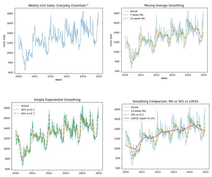
NorthStar RetailGroup monitors weekly sales for its Everyday Essentials™ product line. Weekly sales fluctuate because of promotions, shopping cycles, and ordinary variation in customer behavior. When managers look only at raw sales, it can be difficult to determine whether demand is actually changing or simply moving up and down in the short run.
To clarify direction, NorthStar’s analysts experiment with several smoothing approaches that transform the raw series into decision-ready signals.
Primary dataset: essentials_sales_lite.csv
This simplified dataset contains:
The dataset isolates time and sales so that the effect of smoothing can be seen clearly.
In this SkillBox, you will:
Step 1: Load and Visualize the Time Series
Python
import pandas as pd
import matplotlib.pyplot as plt

df = pd.read_csv("essentials_sales_lite.csv")

plt.plot(df["week_index"], df["sales"], alpha=0.5)
plt.title("Weekly Unit Sales: Everyday Essentials™")
plt.xlabel("Week")
plt.ylabel("Units Sold")
plt.show()
R
df <- read.csv("essentials_sales_lite.csv", stringsAsFactors = FALSE)

str(df)
head(df, 10)

sales_ts <- ts(df$sales, frequency = 52)
plot(sales_ts, main = "Weekly Retail Sales", ylab = "Sales", xlab = "Week")
Interpretive prompt:
Does the series appear mostly stable, or does it show visible short-term volatility that could distract managers?
Step 2: Apply a Simple Moving Average
Use both a 7-period and a 14-period moving average to compare shorter and longer memory.
Python
df["ma_7"] = df["sales"].rolling(window=7).mean()
df["ma_14"] = df["sales"].rolling(window=14).mean()

plt.plot(df["week_index"], df["sales"], alpha=0.4, label="Actual")
plt.plot(df["week_index"], df["ma_7"], "--", label="7-week MA")
plt.plot(df["week_index"], df["ma_14"], "-.", label="14-week MA")
plt.title("Moving Average Smoothing")
plt.xlabel("Week")
plt.ylabel("Units Sold")
plt.legend()
plt.show()
R
library(zoo)

df$ma_7  <- rollmean(df$sales, 7, fill = NA, align = "right")
df$ma_14 <- rollmean(df$sales, 14, fill = NA, align = "right")

plot(df$week_index, df$sales, type = "l", col = "gray60",
     main = "Moving Average Smoothing",
     xlab = "Week", ylab = "Units Sold")
lines(df$week_index, df$ma_7, lty = 2)
lines(df$week_index, df$ma_14, lty = 3)
legend("topleft", legend = c("Actual", "7-week MA", "14-week MA"),
       lty = c(1, 2, 3), bty = "n")
Interpretive prompt:
Which moving average is smoother? Which one reacts faster to changes? Which would be easier for managers to trust?
Step 3: Apply Simple Exponential Smoothing
Use two values of α: 0.2 and 0.7.
Python
from statsmodels.tsa.holtwinters import SimpleExpSmoothing

ses_low = SimpleExpSmoothing(df["sales"]).fit(smoothing_level=0.2, optimized=False)
ses_high = SimpleExpSmoothing(df["sales"]).fit(smoothing_level=0.7, optimized=False)

df["ses_02"] = ses_low.fittedvalues
df["ses_07"] = ses_high.fittedvalues

plt.plot(df["week_index"], df["sales"], alpha=0.4, label="Actual")
plt.plot(df["week_index"], df["ses_02"], "--", label="SES α=0.2")
plt.plot(df["week_index"], df["ses_07"], "-.", label="SES α=0.7")
plt.title("Simple Exponential Smoothing")
plt.xlabel("Week")
plt.ylabel("Units Sold")
plt.legend()
plt.show()
R
library(forecast)

y <- ts(df$sales, frequency = 52)
fit_low  <- ses(y, alpha = 0.2, initial = "simple")
fit_high <- ses(y, alpha = 0.7, initial = "simple")

plot(y, main = "Simple Exponential Smoothing", ylab = "Units Sold", xlab = "Week")
lines(fitted(fit_low), lty = 2)
lines(fitted(fit_high), lty = 3)
legend("topleft", legend = c("Actual", "SES α=0.2", "SES α=0.7"),
       lty = c(1, 2, 3), bty = "n")
Interpretive prompt:
Which signal reacts faster? Which looks more stable? What is the trade-off between early detection and overreaction?
Step 4: Apply LOESS for Visual Comparison
LOESS is included here mainly as a visual comparison tool.
Python
from statsmodels.nonparametric.smoothers_lowess import lowess

df["loess"] = lowess(df["sales"], df["week_index"], frac=0.25, return_sorted=False)

plt.plot(df["week_index"], df["sales"], alpha=0.4, label="Actual")
plt.plot(df["week_index"], df["ma_14"], "--", label="14-week MA")
plt.plot(df["week_index"], df["ses_02"], "-.", label="SES α=0.2")
plt.plot(df["week_index"], df["loess"], label="LOESS (span=0.25)")
plt.title("Smoothing Comparison: MA vs SES vs LOESS")
plt.xlabel("Week")
plt.ylabel("Units Sold")
plt.legend()
plt.show()
R
df$loess <- predict(loess(sales ~ week_index, data = df, span = 0.25))

plot(df$week_index, df$sales, type = "l", col = "gray60",
     main = "Smoothing Comparison: MA vs SES vs LOESS",
     xlab = "Week", ylab = "Units Sold")
lines(df$week_index, df$ma_14, lty = 2)
lines(df$week_index, fitted(fit_low), lty = 3)
lines(df$week_index, df$loess, lty = 1)
legend("topleft", legend = c("Actual", "14-week MA", "SES α=0.2", "LOESS"),
       lty = c(1, 2, 3, 1), bty = "n")
Interpretive prompt:
Which method appears most stable? Which appears most responsive? Which seems most useful for operational interpretation?
By the end of this SkillBox, you should have:
These outputs should help you see how different smoothing methods encode different memory structures and produce different signal behaviors.
This SkillBox shows that the same raw data can produce different signals depending on how memory is designed.
The larger lesson is that smoothing is not mainly about optimizing fit . It is about designing how decision-makers notice change.
Different smoothing methods encode different assumptions about:
A common mistake is to assume that the most responsive signal is automatically the most useful. It is not. A fast-moving signal may detect change earlier, but it may also magnify short-term noise and trigger unnecessary reactions.
Do not judge a smoother only by how dramatic or “smart” it looks on a graph. Ask instead: does this signal help managers respond better, or merely react faster?
There is no universally best smoother. The appropriate design depends on:
Briefly consider:
Submit either:
Your response should focus on signal interpretation and decision usefulness , not coding detail.
You have now seen how different smoothing designs change the signal managers see. The next step is interpretive: how should analysts reason about these differences, especially when AI provides additional explanations?
Using AI as a Learning and Thinking Partner
This LearningLab reinforces the central idea of Chapter 2:
smoothing is not just a technique—it is a design choice about how the past influences the present.
Using AI as both a learning partner and a thinking partner, this LearningLab helps you move from observing variation to structuring how variation is interpreted through time.
The objective is to:
This LearningLab reinforces:
AI is used here to expand reasoning—not to automate smoothing or replace analytical judgment.
In the preceding SkillBox, you applied smoothing methods (such as moving averages and exponential smoothing) to the NorthStar sales data.
You observed that:
This raises a critical insight:
The data has not changed—but what you see depends on how you remember the past.
This LearningLab helps you move beyond applying smoothing methods to understanding their implications:
AI is used here to:
Important principle:
Smoothing does not reveal truth—it constructs a signal based on design choices.
NorthStar analysts have generated multiple smoothed versions of weekly sales using different methods.
Each version tells a slightly different story:
This creates a practical dilemma:
At this stage, the goal is not to select the “best” method, but to understand:
How memory design changes interpretation—and therefore changes decisions.
To support this, analysts use AI to explore and challenge their understanding of smoothing behavior.
You will engage with AI in three structured modes:
Reinforce → Extend → Explore
Work through them in order. Each mode builds a different layer of understanding and expansion.
Build a clear and intuitive understanding of smoothing as temporal memory.
Start your prompt by providing key concepts from the chapter as shown below, then follow with one of the listed prompts or your own chapter-related prompts. This ensures that AI responses align with and reinforce the chapter’s coverage.
Repeating the quiz prompt will generate additional quiz questions.
“Key Concepts from This Chapter
“I understand how smoothing represents different ways of remembering the past.”
Examine how different smoothing methods produce different signals—and why.
Optionally explore additional analytical concepts or methods that interest you but not covered in the chapter.
“I understand how smoothing choices affect the signal I observe and interpret.”
Connect smoothing design to decision consequences.
This is where smoothing becomes part of a decision system, not just a data transformation.
“I understand how smoothing design influences decisions, not just analysis.”
After completing all three modes:
The goal is to evaluate reasoning—not outsource it.
Prepare a short written summary (200–300 words) describing:
You must:
Principle:
AI expands analytical range, but does not replace analytical responsibility.
Smoothing methods differ not in complexity, but in how they encode memory:
These are not just technical differences—they reflect different assumptions about time and relevance.
Insight:
In forecasting, how you remember the past determines how you interpret the present.
You have now moved from:
interpreting patterns → shaping signals
The next step is:
shaping signals → designing decisions
How should different smoothing behaviors translate into:
The DesignStudio will move from:
analytical output → decision design
From Smoothed Data to Operational Action
This DesignStudio moves from analysis to decision system design. You have seen how smoothing changes the signal. You have used AI to reason about those changes. Now you must design a practical signal system that NorthStar managers can interpret consistently and act on responsibly.
This component primarily reinforces Decision Design.
NorthStar monitors weekly sales for its Everyday Essentials™ product line. The analytics team has already created several smoothing signals:
These signals differ in responsiveness and stability, even though they are based on the same data.
Managers use these signals to guide:
Design a directional signal system that helps managers answer:
Is demand meaningfully changing, or are we observing normal variation?
Your design must balance:
NorthStar provides:
Operational constraints include:
Prepare a structured proposal addressing the following:
Prepare a 400–600 word decision design memo to NorthStar’s operations leadership.
Your work will be evaluated on:
A strong response will:
Forecasting methods generate signals. Decision design determines whether those signals create value. A modest method used within a clear decision system is often more useful than a sophisticated method that managers do not understand or trust.
Consider:
You have now designed a signal system for NorthStar. The next step is to apply signal-based reasoning in a different environment where demand is more fragile, external conditions matter more, and the cost of error is less forgiving.
Applying Directional Demand Signals in a New Context
FreshWay Markets is a regional grocery chain that manages perishable inventory across 60 stores. Unlike NorthStar’s relatively stable product category, FreshWay’s demand is highly sensitive to weather, short-term promotions, and spoilage risk.
Produce orders must be placed two days in advance. Overstocking leads directly to waste. Under-ordering leads to lost sales and empty shelves.
FreshWay has adopted a smoothed demand signal based on historical sales, but store managers remain uncertain about how to use it. The signal has trended upward over the past two weeks, yet daily sales remain volatile.
You are the regional operations manager. You must decide whether FreshWay should increase, decrease, or maintain current produce orders for the coming week.
You are given the following:
Prepare a short recommendation that addresses:
Write a 250–400 word memo to the regional supply chain director.
Your memo must:
Focus on:
Consider:
Forecasts do not eliminate uncertainty—they structure it. Good decision-makers act not because signals are perfect, but because they understand how to interpret them in context and manage the risks of being wrong.
Smoothing helps analysts transform noisy observations into directional signals by controlling how much the past influences the present. Different smoothing methods therefore produce different balances of responsiveness, stability, and interpretability. When those balances align with decision needs, smoothing supports better organizational judgment rather than mechanical reaction.
NorthStar’s analytics team has now added smoothing signals to its weekly demand-monitoring dashboard. Moving averages provide a stable planning signal that helps managers avoid overreacting to short-term volatility, while exponential smoothing provides a more responsive signal that can surface emerging shifts earlier. By comparing these signals side by side, NorthStar has begun treating smoothing not merely as a forecasting technique, but as a design choice about how quickly the organization learns from new information. This moves the company from simply observing structure toward understanding forecast behavior and managerial trust. In the next chapter, NorthStar will confront a deeper challenge: what happens when demand itself begins to evolve through trend rather than short-term fluctuation alone?
Reasoning About Responsiveness, Stability, and Decisions
When answering, explain your reasoning clearly. Distinguish signal from noise. Connect analysis to decision consequences. Avoid purely technical answers that ignore managerial context.
Explain:
Here are the three most important ideas from this chapter:
Decision insight: A useful signal is not the one that looks most sophisticated; it is the one that helps the organization respond at the right speed.
Common mistake: Treating the most responsive signal as automatically the best one. Fast signals can create false alarms if they react too strongly to noise.
Smoothing helps organizations see short-term direction, but it does not fully explain what happens when demand itself begins to evolve in a more systematic way. A smoothed signal can reveal movement, yet it does not explicitly model whether that movement reflects a developing trend, a structural shift, or something more persistent in the data.
That unresolved problem leads directly to the next chapter. If smoothing helps us see direction, the next step is learning how to model changing direction more explicitly.

