Forecasting Systems in the Age of AI
Extending Structure with Machine Learning and Generative Reasoning
When forecasting environments become faster, noisier, and more interconnected, the problem is no longer simply how to predict better. It is how to preserve judgment when the system learns patterns faster than humans can explain them.
In classical forecasting, structure is visible. Analysts specify trend, seasonality, and dependence, then test whether those assumptions hold. In AI-era forecasting, some of that structure becomes learned rather than explicitly designed. This creates new power, but also new risk. A system may react faster, fit more signals, and generate richer scenarios—while becoming harder to interpret, govern, and trust.
That is why this chapter matters. The question is not whether AI is more advanced than classical forecasting. The question is whether a forecasting system in the age of AI still supports accountable decisions under uncertainty.
Earlier chapters established a clear progression in forecasting by design. Chapter 2 showed how smoothing creates fast, interpretable signals. Chapter 3 showed how decomposition helps analysts see structure in time before modeling begins. Chapters 4 and 5 formalized visible and hidden temporal structure through explicit modeling choices. Chapter 6 then shifted attention from model fit alone to forecast behavior, trust, diagnostics, and evolution over time.
This chapter extends that logic into the age of AI. As organizations collect richer data and operate in faster decision environments, they increasingly use machine learning, deep learning, and generative AI to extend forecasting capability. But these tools do not eliminate the need for structure. They relocate it. Instead of being fully specified by analysts, structure may now be learned from data, embedded in features, or hidden inside model representations.
A useful analogy is this: classical forecasting is like building with transparent glass walls. You can see the support beams, inspect the cracks, and understand why the structure stands. AI-enhanced forecasting is often more like building with smart materials. The structure can adapt, flex, and respond to the environment—but some of its workings are no longer fully visible. That does not make it unusable. It means the designer must become more deliberate about monitoring, safeguards, and accountability.
This chapter therefore treats AI as an extension of forecasting systems, not as a replacement for forecasting logic. The emphasis remains consistent with this book’s philosophy: forecasting is a decision-support system, not a prediction contest. The goal is not to crown the smartest algorithm. The goal is to decide where structure should remain explicit, where learning adds value, and how human judgment remains responsible when foresight is increasingly shared with machines.
This chapter follows the Forecast-by-Design reasoning progression:
Observe → Understand → Practice → Reason → Design → Decide → Integrate → Consolidate → Continue
The learning flow unfolds as follows:
This chapter is designed as a continuous reasoning system. Each component prepares the next.
After completing this chapter, students will be able to:
When structure is increasingly learned rather than fully specified, how should organizations design forecasting systems that remain interpretable, governable, and decision-useful over time?
In September 2021, Netflix released Squid Game with no expectation that it would become a global phenomenon on the scale that followed. Within days, viewership surged across continents. Social media attention exploded across languages and markets where the series had not been heavily promoted. Subscriber activity shifted in places that had previously appeared stable, mature, or even saturated.
From a forecasting perspective, the pattern did not behave like the familiar problems studied in earlier business settings. Historical trend gave little warning. Seasonality offered little explanation. The shock was not random noise, and it did not quickly fade back to normal. Instead, demand spread through networks of attention, social imitation, and cultural diffusion. It behaved less like a temporary spike and more like a wave moving through an interconnected system.
This did not mean forecasting had failed. It meant the forecasting environment had changed.
For much of its earlier history, Netflix operated in a world where classical forecasting often worked well enough. Subscriber growth followed a visible trajectory. Weekly rhythms were recognizable. Seasonal effects recurred with reasonable regularity. Trend-based models, seasonal adjustments, and structured time-series methods provided useful planning signals. The models were not perfect, but they were interpretable, stable, and decision-ready.
As Netflix evolved into a global streaming platform, however, the nature of demand changed. Content releases became strategic shocks. External signals such as search activity and social media began leading consumption rather than merely reflecting it. Leaders no longer wanted only a point forecast. They wanted to ask counterfactual questions: What happens if a release is delayed? What if competitor timing changes? What if promotional intensity rises in one region and not another? What if the surge spreads faster than historical patterns suggest?
At that point, forecasting stopped being only a modeling problem. It became a system design problem.
A useful analogy is weather forecasting. A simple local forecast might be enough when yesterday looks much like today. But when a hurricane forms, forecasters do not rely on one curve and one number. They monitor multiple models, track disagreement, update scenarios, and communicate risk bands to decision-makers. The challenge is not merely prediction. It is designing a system that helps people act responsibly under uncertainty.
That is the turning point this chapter examines. In the age of AI, forecasting systems must do more than extrapolate the past. They must combine explicit structure, learned structure, and human judgment in ways that preserve trust. Structure → Behavior → Trust still matters. The tools change, but the design responsibility remains.
The progression developed across earlier chapters now reaches its next stage. In classical forecasting, the analyst specifies how time matters. Trend may be modeled explicitly. Seasonality may be decomposed. Dependence may be represented through lag structures and residual correction. These models make structure visible. They allow analysts to inspect assumptions, diagnose failures, and explain why forecasts behave the way they do.
AI-era forecasting changes where this structure lives.
Instead of fully specifying how the past should influence the future, analysts may now provide richer inputs and let algorithms learn patterns from data. This does not eliminate structure. It relocates it. Some structure still remains explicit in features, holdout design, and system rules. Some becomes embedded inside models. As a result, the analyst’s role shifts from only fitting models to designing the forecasting system within which different models operate.
This chapter therefore builds on the full spine of the book:
That spine matters even more in AI settings because complexity can create the illusion that judgment is no longer necessary. But models don’t decide—systems do. And systems still require human responsibility.
If organizations treat AI forecasting as a technical upgrade rather than a design question, they risk overreacting to noise, underexplaining critical assumptions, and delegating accountability to tools that cannot own consequences.
A common mistake is to compare AI-era methods only by average error. That is like judging a vehicle only by top speed while ignoring steering, braking, and visibility. In decision contexts, forecast behavior matters as much as forecast fit.
At NorthStar Retail Group, weekly unit sales for Everyday Essentials™ are influenced not only by recurring seasonal patterns but also by promotions, holidays, and occasional shocks in demand. A structurally explicit model may describe the baseline well. But when promotion intensity changes or consumer attention shifts unexpectedly, a more adaptive model may respond faster. The challenge is deciding whether that responsiveness reflects meaningful signal or temporary noise.
To understand that trade-off, we first need to clarify what statistical learning emphasizes, what machine learning adds, and what deep learning changes.
The methods developed earlier in this book—smoothing, decomposition, and ARIMA-style modeling—belong to a broader family of statistical learning approaches. Their shared philosophy is simple but powerful: begin with interpretable structure, then fit parameters within that structure.
The Box–Jenkins tradition makes this especially clear through three coordinated steps:
These models matter in forecasting by design not because they always maximize accuracy, but because they make assumptions inspectable. They help analysts explain what the model is doing, where it may fail, and why the forecast should or should not be trusted.
A useful analogy is bridge engineering. A well-designed bridge is not judged only by whether it stands today. It is judged by whether engineers understand the forces it was designed to withstand, how stress is distributed, and what warning signs indicate weakness. Statistical learning has this same virtue. It makes structural reasoning visible.
This is why classical models remain important even in AI-era environments. They provide interpretive scaffolding, diagnostic anchors, and trustworthy baselines.
Students often assume classical methods are “older” and therefore less relevant. But in practice, older methods frequently remain valuable precisely because they are explainable and stable.
When leaders must justify a forecast to others, visible structure is an asset, not a limitation.
Machine-learning forecasting models reframe the forecasting problem. Instead of beginning with a fully specified statistical structure for how data evolve over time, they often begin with a prediction task and then learn relationships from data through training.
That difference is important. In statistical learning, the analyst usually designs the structure first, such as a quadratic trend with 12-month seasonality, and estimates within it. In machine learning, the analyst still designs the system—but in a different way. The design work shifts away from writing model equations and toward choices such as:
In other words, machine learning does not eliminate design. It relocates it.
Machine learning adds flexibility in settings where demand is shaped by many interacting signals and where those relationships are difficult to specify in advance. This is especially valuable when:
A classical model may represent time directly through trend, seasonality, and dependence. A machine-learning model can instead learn that the effect of one variable depends on the level of another, or that the same promotion behaves differently in different calendar periods or demand regimes.
For example, in retail forecasting, a statistical model might represent sales as a combination of baseline trend, seasonal rhythm, and error. A machine-learning model might discover a more conditional pattern: a promotion increases sales strongly when inventory has been stable for several weeks, but the same promotion has much less effect when it occurs immediately after a holiday surge or during a period of already elevated demand. The analyst did not write that rule explicitly. The model learned it from historical examples.
This ability to learn interactions is one of machine learning’s main contributions.
To understand machine learning in forecasting, students need a tangible idea of feature engineering , because feature engineering is one of the most important design tasks in these systems.
A feature is simply an input (predictor) the model uses to make a prediction. In forecasting, raw time itself is usually not enough. The analyst often must create features ( feature engineering) that help the model “see” temporal structure. These may include:
Feature engineering matters because many machine-learning models do not understand time naturally. They do not automatically know that last week should matter more than last year, or that December holiday demand differs from a routine week in March. The analyst must decide how time and context will be represented.
A useful analogy is this: statistical forecasting is like giving a model a carefully drawn blueprint of the building. Machine learning is more like giving the system a box of building materials and examples of finished structures. The model can learn powerful patterns, but only if the materials are relevant and well prepared. Feature engineering is the work of preparing those materials.
The added flexibility of machine learning comes with trade-offs. As flexibility increases, interpretability often decreases. Relationships may be learned without being easily explained in business language. Hidden assumptions begin to replace visible ones.
In a statistical model, assumptions are usually explicit: the analyst states a trend form, a seasonal pattern, or a dependence structure. In machine learning, assumptions still exist, but they often appear in less visible places:
This means machine learning can create an illusion of objectivity: the model appears to “discover” truth directly from data, when in fact the system reflects many human design choices.
Suppose two analysts both use a machine learning algorithm (e.g. gradient boosting) on the same weekly sales data.
Even though they are using the same algorithm, they have effectively designed two very different forecasting systems. The second system may perform much better—not because the algorithm is smarter, but because the time structure was represented more thoughtfully.
This is a core lesson of forecasting in the age of AI: with machine learning, the design burden often moves upstream.
Seen this way, machine learning does not replace statistical learning. It extends it.
Statistical learning gives us discipline:
Machine learning adds:
Neither is universally better. They serve different purposes.
That distinction matters because it clarifies what each approach contributes. Statistical learning emphasizes explicit temporal logic. Machine learning emphasizes learned predictive relationships.
The right choice depends on decision context.
If the forecast supports routine replenishment, managers may value stability, interpretability, and trust. If the forecast supports disruption detection or rapid response, they may value faster adaptation and sensitivity to emerging signals.
A forecasting system that is excellent for one purpose may be poorly suited to another.
A common mistake is to believe that machine learning removes assumptions. It does not. It moves assumptions from model equations into system design choices such as feature engineering, validation, and training setup.
That is why machine-learning forecasts require disciplined governance. When structure becomes less visible, responsibility must become more deliberate.
This becomes even clearer when we compare how different forecasting families represent time itself: explicitly through model structure, indirectly through engineered features, or implicitly through learned memory.
A common misconception is that machine learning and AI make classical forecasting obsolete. In practice, modern forecasting systems usually become layered, not replaced.
Classical models often continue to serve as:
Machine-learning models may then extend the system by capturing nonlinear effects, richer external signals, or faster changes. Deep-learning models may serve as specialized tools in settings with large data volumes and strong sequence structure. Generative AI may then add a further layer by helping humans interpret disagreement, stress-test assumptions, and communicate scenarios.
This is why the correct question is not “Which model wins?” but “How should different models be positioned within a forecasting system designed for specific decision stakes?”
When students frame the chapter as a competition between classical and AI methods, they miss the deeper lesson. The forecasting problem has changed from single-model choice to governed system design.
To make that shift concrete, we now compare four forecasting approaches using the same logic and the same NorthStar decision setting.
Prophet, Boosting, and LSTM
Section 7.1 established the central shift of this chapter: as forecasting systems evolve, structure moves from being fully specified by analysts to being increasingly learned from data. This section makes that shift concrete by comparing four approaches that occupy different positions on that spectrum:
All four approaches are examined within the same NorthStar context, allowing students to observe differences in behavior rather than rely on abstract labels. This comparison emphasizes how each approach represents, learns, and utilizes structure.
Understanding these differences shifts the question from “Which model is best?” to “How should forecasting systems be designed and governed under different forms of learned structure?”
SARIMA remains important because it represents time explicitly. Trend and seasonality are not hidden. Dependence is modeled through interpretable lag structure and seasonal correction. This makes SARIMA especially useful as a baseline and diagnostic reference.
Managerial analogy: SARIMA is like a well-calibrated compass. It may not tell you everything about the terrain, but it gives you a stable reference point. When other signals shift, the compass helps you see whether the change is real or only apparent.
SARIMA is most useful when historical structure remains meaningful and the organization needs a forecast that can be explained, monitored, and defended.
It can adapt slowly when the environment changes quickly or when shocks are driven by forces not well represented in past time structure.
Prophet sits between classical statistical forecasting and more automated AI-era methods. It preserves the additive intuition of decomposition while allowing key components—especially trend—to adjust more flexibly through automated changepoints and business-friendly defaults.
To understand Prophet clearly, it helps to relate it directly to the decomposition models introduced earlier.
In Chapter 3, decomposition was introduced as a way to represent time series structure:
where:
This formulation is descriptive and interpretive. It helps analysts see structure, but it does not specify how that structure evolves over time or how it should be forecast.
Prophet extends this idea into a modeling and forecasting system:
where
At first glance, this looks very similar to decomposition. That similarity is intentional. Prophet keeps structure visible and interpretable.
Prophet retains three key principles from classical decomposition:
In this sense, Prophet behaves like a “smart decomposition model”—it keeps the interpretability of decomposition while turning it into a forecasting engine.
The key difference is not the structure itself, but how that structure evolves.
1. Flexible Trend via Changepoints
In classical decomposition, trend is often assumed to be smooth or slowly varying. Prophet instead allows:
g(t) = piecewise trend with changepoints
This means the model can automatically detect moments where growth accelerates, slows down, or shifts direction.
Example (Business intuition):
If a retailer suddenly expands distribution or changes pricing strategy, the growth pattern may shift. A classical trend might adjust slowly. Prophet can introduce a changepoint where the slope changes more quickly.
2. Systematic Seasonality Representation
Instead of manually specifying seasonal patterns, Prophet models seasonality using flexible functions (e.g., Fourier series):
This allows:
Difference from decomposition:
Classical decomposition estimates seasonality directly from averages. Prophet parameterizes it, making it easier to extend and automate.
3. Explicit Event Effects
Prophet introduces a separate component:
to capture known events such as promotions or holidays.
In classical decomposition, such effects often appear inside the residual R t . Prophet instead pulls them out explicitly, making them visible and controllable.
Example:
A promotion week is not treated as noise—it is treated as a structured, explainable driver.
The most important distinction is this:
A useful analogy:
Prophet is like a smart autopilot.
This balance between visibility and adaptability is what makes Prophet attractive in business settings.
Prophet often works well when:
It provides a middle ground:
Because Prophet automates flexibility—especially through changepoints—there is a risk of over-trusting detected changes.
Not every detected shift represents a durable structural change. Some may reflect:
If analysts accept every adjustment without questioning its cause, they may confuse reactivity with understanding.
Prophet is most valuable when organizations need forecasts that are:
But its outputs still require judgment.
In forecasting by design:
This middle position—between explicit structure and learned flexibility—helps clarify the broader comparison. As we move to feature-based machine learning and deep learning, structure becomes less visible and more implicit, shifting even more responsibility onto system design and validation.
Gradient boosting changes the language of forecasting. Instead of modeling time directly through explicit dependence structures, it reframes forecasting as a supervised learning problem:
where:
This formulation is fundamentally different from classical time-series models. Time is no longer modeled through equations of dependence. It is represented indirectly through features.
Gradient boosting builds a model as a sequence of small decision trees:
where:
The result is an ensemble model that can capture complex, nonlinear relationships and interactions across features.
Importantly, the model does not “know time” unless time is encoded in X t .
In boosting, feature design becomes model design.
To forecast y t , the analyst constructs X t using information available up to time ttt. Common feature types include:
(to approximate short-term and seasonal memory)
(to smooth recent behavior)
These features are how the model “sees” time.
If the features are incomplete, the model’s understanding of time is incomplete.
Gradient boosting adds flexibility in three important ways:
A classical model might assume promotions increase demand by a consistent amount.
A boosting model might learn:
This conditional behavior is difficult to specify explicitly but can be learned through data.
The flexibility of boosting comes with important trade-offs:
Classical models are like a well-defined equation describing how time behaves.
Gradient boosting is more like a dashboard of signals. The system learns how to combine them, but the logic is distributed across many small decisions rather than a single interpretable structure.
This is a fundamental shift:
Boosting is especially useful in operational settings where:
However, this responsiveness comes with volatility risk. A model that reacts quickly may also react to noise.
Therefore:
A critical error in applying boosting to time series is incorrect validation design.
Using random train-test splits breaks temporal order and allows the model to “see the future.” This leads to overly optimistic performance estimates.
Correct validation must be time-aware, such as:
If validation leaks future information:
Gradient boosting does not eliminate temporal structure—it shifts it into:
In forecasting by design, this means:
This feature-based view of time sits between classical models and deep learning. In the next section, we examine LSTM models, where time is no longer engineered or specified—but learned as an internal representation.
If gradient boosting learns from hand-crafted summaries of time, LSTM (Long Short-Term Memory) models go further by learning sequence structure directly from historical data. Instead of specifying which lags matter or constructing features explicitly, the analyst provides sequences of past observations, and the model learns how to represent temporal dependence internally.
Formally, an LSTM produces forecasts of the form:
where:
Internally, the model maintains a hidden state (memory):
This hidden state h t evolves over time and determines what information is retained, updated, or forgotten.
The analyst does not decide which lags matter. The model learns what to remember.
LSTM models add a fundamentally different capability: they can learn long-range, nonlinear temporal dependencies without requiring explicit specification.
This is especially valuable when:
Consider demand influenced by a sequence of events:
A classical model may struggle to capture this delayed, multi-stage effect unless explicitly specified. A boosting model may approximate it through carefully engineered lags. An LSTM can learn this pattern directly from sequences—if enough data exist.
Unlike classical models or feature-based approaches, LSTM does not treat time as a set of variables. It treats time as a flow of information.
At each step, the model decides:
This process is controlled by internal mechanisms (often called “gates”), which regulate memory flow.
If statistical models are like writing rules and boosting is like combining signals, LSTM is like learning from experience directly.
Instead of saying:
the model learns:
The rules are not written—they are encoded in the learned representation.
The main trade-off is loss of visibility into structure.
In classical models, if forecasts behave unexpectedly, analysts can inspect parameters or residuals. In LSTM, unexpected behavior may be buried inside learned representations.
LSTMs are not the default next step after classical forecasting. They are specialized tools.
They are most appropriate when:
They are less appropriate when:
In such cases, LSTMs may create fragile sophistication—models that appear advanced but add little reliable decision value.
As we move from left to right:
LSTMs can add value in specialized environments, such as:
However, they should rarely be used in isolation.
In most business settings, LSTMs are best positioned as:
rather than primary decision anchors.
Common pitfalls include:
Because structure is implicit, these issues are harder to diagnose early.
The greatest risk of LSTM is the illusion of intelligence.
The model may produce smooth, plausible forecasts that appear sophisticated, but:
In forecasting by design, LSTM does not remove the need for structure. It increases the need for disciplined system design.
This includes:
LSTM does not eliminate forecasting structure.
It relocates structure into learned representations.
As structure becomes less visible, the responsibility to design, validate, and govern the forecasting system becomes more important—not less.
With SARIMA, Prophet, boosting, and LSTM now positioned along a spectrum from explicit to learned structure, the next step is to compare them within a single decision setting—so that differences in behavior become visible and actionable.
A disciplined comparison does not ask which model is “best” in the abstract. It asks how each model behaves under the same decision setting.
Across the same NorthStar dataset and the same time-aware holdout design, the key questions are:
This is why the chapter compares models not only by metrics, but by where structure lives and how responsibility is shared.
|
Dimension |
SARIMA |
Prophet |
Gradient Boosting |
LSTM |
|---|---|---|---|---|
|
How time is represented |
Explicit dependence and seasonality |
Explicit components with automated changepoints |
Time encoded through features |
Time learned through sequences |
|
Where structure lives |
Specified by analyst |
Mostly specified, partly automated |
Learned from features and data |
Learned largely inside the model |
|
Interpretability |
High |
High to moderate |
Moderate to low |
Low |
|
Responsiveness |
Slower |
Moderate |
Often high |
Potentially high, but unstable |
|
Data requirements |
Low to moderate |
Moderate |
Moderate to high |
High |
|
Role in system |
Baseline and diagnostic anchor |
Explainable deployable forecast |
Complementary adaptive signal |
Specialized extension |
|
Primary risk |
Missing breaks |
Overtrust in automated shifts |
Overfitting noisy features |
Illusion of intelligence |
AI does not eliminate forecasting structure. It relocates it. The design question is where structure should live and who remains accountable when it moves.
From Model Selection to System Design
The comparison above leads to a practical conclusion: no single forecasting method is best in all environments. Each method makes some risks easier to see and some risks easier to hide.
This is not a limitation of modeling—it is a property of decision-making under uncertainty.
As a result, modern forecasting practice is shifting away from selecting a single “best” model and toward designing systems of models.
Hybrid systems combine complementary model roles. Generative AI then helps humans interpret disagreement, organize scenarios, and communicate choices. Together, they move forecasting from model selection toward governed decision systems.
Hybrid forecasting emerged not because it is fashionable, but because operational environments became too complex for one model family to handle well under all conditions.
Each of these approaches contributes something valuable. None of them is sufficient on its own.
A hybrid forecasting system is like a medical team. A general practitioner provides continuity and baseline judgment. Specialists contribute deeper expertise when needed. No one assumes that the most sophisticated specialist should handle every problem alone. Good care comes from designed coordination.
If an organization relies on only one forecasting approach, it concentrates risk.
A hybrid system distributes that risk across complementary strengths.
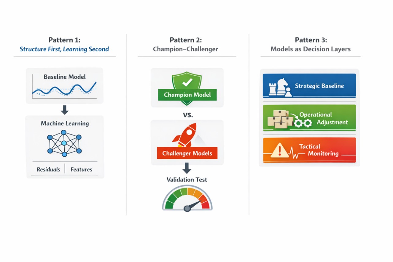
Hybrid systems do not emerge randomly. In practice, they tend to follow a small number of recurring design patterns.
These patterns differ in how models interact, how decisions are made, and how change is governed.
A structured statistical model is first used to capture the core components of the series, such as trend and seasonality. Machine learning methods are then applied to:
This design prevents flexible learning systems from inefficiently rediscovering basic structure and focuses their capacity on what remains unexplained.
Design Logic
Let structure handle what is stable and visible.
Let learning focus on what is complex or context-dependent.
Strengths
Limitations
Typical Use
A stable “champion” model serves as the baseline forecast. More adaptive “challenger” models are continuously evaluated using forward validation.
Challengers are promoted only when they demonstrate consistent and reliable improvement over time, not just temporary gains.
Design Logic
Change is earned through evidence, not novelty.
Strengths
Limitations
Typical Use
The first two patterns still treat forecasting primarily as a model selection problem . Pattern 3 introduces a different perspective:
Multiple models are not competitors—they are designed as a system to support different decisions .
Instead of choosing one model, Pattern 3 organizes models into decision layers , where each model reacts differently to changes in the data. A classical model may smooth over short-term fluctuations and emphasize long-term stability. A machine-learning model may respond quickly to recent signals, amplifying both meaningful changes and transient noise. A deep-learning model may capture complex patterns that are difficult to articulate but may also become unstable when data are limited or conditions shift. Each model contributes to a different level of action.
When these models are viewed together, their differences become informative. If all models move in the same direction, confidence in that signal increases. If one model reacts sharply while others remain stable, the discrepancy itself becomes a signal that something may be changing—or that noise is being amplified.
At NorthStar Retail Group, for example, weekly sales forecasts generated by different models may not align. A SARIMA model might suggest stable continuation. A boosting model might indicate a sharp increase driven by recent signals. A Prophet model might show a gradual upward shift reflecting a structural change. Rather than forcing these forecasts into agreement, analysts interpret them as alternative representations of the system.
In this context, disagreement is not a problem to be solved. It is evidence to be understood.
Chapter 6 introduced forward validation and residual signals for deciding whether to maintain, refit, or rethink a model.
The practical value of hybrid systems becomes most visible when forecasts are linked directly to decisions.
Traditional forecasting often presents results in the form of point estimates and confidence intervals. While these outputs are statistically meaningful, they are not always sufficient for operational decision-making. Managers do not act on intervals alone. They act on conditions.
Hybrid systems support a different approach. Instead of asking what the forecast is, organizations ask when action should be taken.
This leads to trigger-based decision design.
Consider an inventory planning scenario. If all models indicate stable demand, the appropriate action may be to maintain current plans. If a more adaptive model begins to signal an increase while others remain unchanged, the organization may choose to monitor the situation more closely rather than act immediately. If multiple models begin to indicate rising demand, the evidence becomes stronger, and adjustments to inventory or staffing may be warranted. If residual signals indicate instability or structural change, escalation may be necessary.
In this way, forecasts are not treated as answers. They are treated as inputs into a decision process that defines when to maintain, adapt, or escalate.
A useful analogy is weather forecasting. When a storm approaches, forecasters do not rely on a single projected path. They monitor multiple models, observe how those paths evolve, and issue advisories based on thresholds of risk. The goal is not to predict the exact trajectory, but to enable timely and responsible action.
Hybrid forecasting systems bring this same logic into business settings. They transform forecasts from static outputs into dynamic decision signals.
At NorthStar RetailGroup, forecasting supports multiple decision horizons:
A hybrid system assigns models accordingly:
|
Decision Layer |
Model Role |
Typical Model |
Behavior Emphasis |
Decision Use |
|---|---|---|---|---|
|
Strategic (Slow-moving) |
Baseline Stability |
SARIMA / trend models |
Stable, interpretable |
Capacity, budgeting |
|
Operational (Adaptive) |
Signal Adjustment |
Prophet / Gradient Boosting |
Responsive to recent changes |
Staffing, inventory |
|
Tactical (Fast-response) |
Early Warning |
LSTM / residual monitoring |
Sensitive to anomalies |
Alerts, escalation |
Each model is evaluated based on its fitness for purpose, not global dominance.
In Pattern 3, residuals become decision signals rather than purely diagnostics.
|
Residual Pattern |
Interpretation |
Action |
|---|---|---|
|
Stable variation |
Model adequate |
Maintain |
|
Gradual drift |
Structure shifting |
Refit |
|
Sudden instability |
Regime change |
Rethink / escalate |
These signals may differ across models. Such differences are not errors—they are informative tensions that guide action.
A hybrid decision system allows coordinated responses:
This produces structured logic:
Maintain where structure holds.
Adapt where signals shift.
Escalate where instability emerges.
A common misunderstanding is that hybrid forecasting means averaging models.
In forecasting by design, hybrid means:
assigning roles deliberately across models to support different decisions.
Generative AI plays a different role from numerical forecasting models. It does not replace prediction—it supports interpretation and reasoning.
Used responsibly, generative AI can help teams:
When models disagree, the key question is not “Which is correct?” but:
AI supports reasoning. Humans own decisions.
Generative AI should not be used to declare the “correct” forecast.
That replaces disciplined judgment with narrative confidence.
In AI-era forecasting, the analyst evolves from model builder to system designer.
This includes the ability to:
This approach provides a practically meaningful and actionable complement to conventional single-model, confidence-interval-based forecast regimes.
Technical skill remains essential. But design judgment becomes central.
Through SkillBox 7, you will practice how to obtain and compare the various models for different decision layers. Chapter 8 and the capstone project will demonstrate and apply how a Pattern 3 hybrid decision design is created and used.
As forecasting systems become hybrid, layered, and AI-supported, responsibility extends beyond performance to include explainability, bias, and ethics.
Why Responsibility Is a Design Requirement
As forecasting systems become more sophisticated, the most difficult problems are often no longer algorithmic. They are organizational.
A forecast may be accurate on average and still be unusable if no one can explain it, challenge it, or take responsibility for acting on it. In high-stakes settings, explanation is not optional. It is part of governance.
Forecasts support decisions, coordination, and accountability. Decision-makers must be able to answer basic questions:
Explainability does not require revealing every line of code. It requires enough clarity for the organization to understand the structure, limits, and risks of the forecast.
When forecasts guide staffing, inventory, pricing, capacity, or investment, poor explanation can lead to misuse even if average model performance looks strong.
Bias in forecasting systems often enters through data, feature construction, proxy variables, feedback loops, and organizational use. It is rarely just a property of the model itself.
For example, if past allocation decisions restricted supply in certain regions, the data may reflect constrained demand rather than true demand. If forecasts then learn from those patterns, the system can preserve yesterday’s limitations and present them as tomorrow’s expectation.
Forecasts do not merely describe the future. They can shape it.
Bias is often treated as an ethical add-on rather than a design issue. In forecasting by design, bias is a system issue because forecasts influence action, and action shapes future data.
Before deployment, and throughout continued use, teams should be able to answer:
If these questions cannot be answered, the problem is not merely the algorithm. The problem is the forecasting system.
Responsible AI-supported forecasting belongs to Decision Design, not only to technical modeling.
From Classical Structure to AI-Era Learning Without Losing Decision Readiness
This SkillBox is designed to help students compare forecast behavior, not optimize models. You will evaluate how four forecasting systems respond to the same business data under the same time-aware validation design. The emphasis is on interpretation, decision stakes, and trust.
NorthStar Retail Group is monitoring weekly unit sales for Everyday Essentials™. Promotions and holidays create recurring variations, but some changes are sharper and more difficult to explain through baseline seasonality alone. Leadership wants to understand not only which forecast fits the past, but which forecasting system is most useful for routine planning and which one provides an early warning signal when conditions shift.
Primary dataset: essentials_sales.csv
Core variables include:
Derived variables used inside the workflow may include lagged values, rolling summaries, and calendar features.
NorthStar uses these forecasts to support replenishment, promotion planning, and staffing coordination. If the forecast is too slow, the company may miss a surge. If it is too reactive, it may overcommit inventory and operations to noise.
Using the provided Python or R reference code, you will compare four forecasting systems on the same holdout design:
Your task is not to improve them. Your task is to interpret how they behave.
Python
import pandas as pd
import numpy as np
import matplotlib.pyplot as plt
from statsmodels.tsa.statespace.sarimax import SARIMAX
from prophet import Prophet # Ensure 'prophet' is installed
from sklearn.ensemble import GradientBoostingRegressor
from sklearn.preprocessing import MinMaxScaler
from sklearn.metrics import mean_absolute_error
from tensorflow.keras.models import Sequential
from tensorflow.keras.layers import LSTM, Dense
import warnings

warnings.filterwarnings('ignore')

# 1. Load Data
df = pd.read_csv('essentials_sales.csv')
df['week'] = pd.to_datetime(df['week'])
df = df.sort_values('week')

# 2. Set Holdout to 52 Weeks (One full year)
holdout_size = 52
train = df.iloc[:-holdout_size].copy()
test = df.iloc[-holdout_size:].copy()

plt.figure(figsize=(16, 9))

# Plot Actual Sales
plt.plot(df['week'], df['sales'], label='Actual Sales', color='black', alpha=0.3, lw=1)

# --- Visual Markers for Promotions and Holidays ---
promo = df[df['promotion'] == 1]
holiday = df[df['holiday'] == 1]
plt.scatter(promo['week'], promo['sales'], color='red', marker='^', label='Promotion Event', s=50, zorder=5)
plt.scatter(holiday['week'], holiday['sales'], color='blue', marker='s', label='Holiday Event', s=40, zorder=5)

# --- 1. Baseline SARIMA (Interpretable) ---
exog_cols = ['promotion', 'holiday']
sarima_model = SARIMAX(train['sales'], exog=train[exog_cols],
                       order=(1, 1, 1), seasonal_order=(1, 1, 1, 52))
sarima_fit = sarima_model.fit(disp=False)
sarima_pred = sarima_fit.forecast(steps=holdout_size, exog=test[exog_cols])
plt.plot(test['week'], sarima_pred, label='SARIMA', color='orange', lw=2.5)

# --- 2. Prophet (Structural Flexibility) ---
p_train = train.rename(columns={'week': 'ds', 'sales': 'y'})
p_test = test.rename(columns={'week': 'ds', 'sales': 'y'})
m = Prophet(yearly_seasonality=True, weekly_seasonality=False, daily_seasonality=False)
m.add_regressor('promotion')
m.add_regressor('holiday')
m.fit(p_train)
forecast = m.predict(p_test[['ds', 'promotion', 'holiday']])
plt.plot(test['week'], forecast['yhat'].values, label='Prophet', color='green', lw=2)

# --- 3. Gradient Boosting (GBM - Feature Based) ---
def create_features(data):
    d = data.copy()
    d['month'] = d['week'].dt.month
    d['lag1'] = d['sales'].shift(1)
    d['lag52'] = d['sales'].shift(52) # Capture annual seasonality
    return d

df_f = create_features(df)
train_gbm = df_f.iloc[:-holdout_size].dropna()
test_gbm = df_f.iloc[-holdout_size:]
gbm_features = ['promotion', 'holiday', 'month', 'lag1', 'lag52']

gbm = GradientBoostingRegressor(n_estimators=100, learning_rate=0.1)
gbm.fit(train_gbm[gbm_features], train_gbm['sales'])
gbm_pred = gbm.predict(test_gbm[gbm_features])
plt.plot(test['week'], gbm_pred, label='GBM (Gradient Boosting)', color='purple', ls='--')

# --- 4. LSTM (Deep Learning Demonstration) ---
scaler = MinMaxScaler()
scaled_data = scaler.fit_transform(df[['sales', 'promotion', 'holiday']])

def create_seq(data, window=4):
    X, y = [], []
    for i in range(len(data)-window):
        X.append(data[i:i+window])
        y.append(data[i+window, 0])
    return np.array(X), np.array(y)

window = 4
X, y = create_seq(scaled_data, window)
X_train, X_test = X[:-holdout_size], X[-holdout_size:]
y_train = y[:-holdout_size]

lstm = Sequential([
    LSTM(32, activation='relu', input_shape=(window, 3)),
    Dense(1)
])
lstm.compile(optimizer='adam', loss='mse')
lstm.fit(X_train, y_train, epochs=25, verbose=0)
lstm_p_scaled = lstm.predict(X_test)
# Inverse Scaling
s_min, s_max = df['sales'].min(), df['sales'].max()
lstm_pred = lstm_p_scaled * (s_max - s_min) + s_min
plt.plot(test['week'], lstm_pred, label='LSTM', color='cyan', alpha=0.8)

# Final Plotting Details
plt.axvline(train['week'].iloc[-1], color='gray', linestyle='--', label='Holdout Start')
plt.title('Comparison of Sales Forecast Models (52-Week Holdout)')
plt.legend(loc='upper left', bbox_to_anchor=(1, 1))
plt.grid(True, linestyle=':', alpha=0.6)
plt.tight_layout()
plt.show()
R
suppressWarnings({
  suppressMessages({
    library(readr)
    library(dplyr)
    library(lubridate)
    library(ggplot2)
    library(forecast)
    library(gbm)
    library(scales)
    library(keras3)
  })
})
DATA_PATH <- "C:/temp/essentials_sales.csv"   # set path if needed
holdout_size <- 52

# ---------------------------
# 1) Load Data
# ---------------------------
df <- read_csv(DATA_PATH, show_col_types = FALSE) %>%
  mutate(
    week = as.Date(week, format = "%m/%d/%Y"),
    sales = as.numeric(sales),
    promotion = as.numeric(promotion),
    holiday = as.numeric(holiday)
  ) %>%
  arrange(week)

train <- df %>% slice(1:(n() - holdout_size))
test  <- df %>% slice((n() - holdout_size + 1):n())
# ---- 1) Basic cleaning / guards ----
# Replace missing event flags with 0
train <- train %>% mutate(
  promotion = ifelse(is.na(promotion), 0, promotion),
  holiday   = ifelse(is.na(holiday), 0, holiday)
)
test <- test %>% mutate(
  promotion = ifelse(is.na(promotion), 0, promotion),
  holiday   = ifelse(is.na(holiday), 0, holiday)
)

# Ensure sales has no NA/Inf in training
train <- train %>% filter(is.finite(sales))
stopifnot(nrow(train) > 2 * 52)  # rule-of-thumb: need enough data for seasonal modeling

y_train <- ts(train$sales, frequency = 52)

xreg_train <- as.matrix(train %>% select(promotion, holiday))
xreg_test  <- as.matrix(test  %>% select(promotion, holiday))

# Force finite values (just in case)
xreg_train[!is.finite(xreg_train)] <- 0
xreg_test[!is.finite(xreg_test)] <- 0

# ---- 2) If regressors are constant, drop them to avoid instability ----
const_cols <- apply(xreg_train, 2, function(x) sd(x) == 0)
if (any(const_cols)) {
  message("Dropping constant xreg columns: ", paste(colnames(xreg_train)[const_cols], collapse = ", "))
  xreg_train <- xreg_train[, !const_cols, drop = FALSE]
  xreg_test  <- xreg_test[,  !const_cols, drop = FALSE]
}

# ---- 3) Robust fit with tryCatch + fallback ----
fit_sarima <- tryCatch(
  {
    auto.arima(
      y_train,
      xreg = if (ncol(xreg_train) > 0) xreg_train else NULL,
      seasonal = TRUE,
      stepwise = TRUE,          # safer / more stable than exhaustive search
      approximation = FALSE,
      method = "ML"             # more stable than CSS-ML in some cases
    )
  },
  error = function(e) {
    message("SARIMA with xreg failed; refitting without xreg. Reason: ", e$message)
    auto.arima(
      y_train,
      seasonal = TRUE,
      stepwise = TRUE,
      approximation = FALSE,
      method = "ML"
    )
  }
)

fc_sarima <- forecast(
  fit_sarima,
  h = HOLDOUT_WEEKS,
  xreg = if (!is.null(fit_sarima$xreg)) xreg_test else NULL
)$mean %>% as.numeric()
sarima_pred <- as.numeric(forecast(fit_sarima, h = holdout_size, xreg = xreg_test)$mean)

# ---------------------------
# --- 2. Prophet (Structural Flexibility) ---
# ---------------------------
prophet_pred <- rep(NA_real_, holdout_size)
if (requireNamespace("prophet", quietly = TRUE)) {
  suppressMessages(library(prophet))

  p_train <- train %>% transmute(ds = week, y = sales, promotion = promotion, holiday = holiday)
  p_test  <- test  %>% transmute(ds = week, y = sales, promotion = promotion, holiday = holiday)

  m <- prophet(
    yearly.seasonality = TRUE,
    weekly.seasonality = FALSE,
    daily.seasonality  = FALSE
  )
  m <- add_regressor(m, "promotion")
  m <- add_regressor(m, "holiday")

  m <- fit.prophet(m, p_train)

  fc <- predict(m, p_test %>% select(ds, promotion, holiday))
  prophet_pred <- as.numeric(fc$yhat)
} else {
  message("Prophet not installed. Run: install.packages('prophet')")
}

# ---------------------------
# --- 3. Gradient Boosting (GBM - Feature Based) ---
# Python features: month, lag1, lag52 + promotion/holiday
# ---------------------------
create_features <- function(data) {
  d <- data %>%
    mutate(
      month = month(week),
      lag1  = dplyr::lag(sales, 1),
      lag52 = dplyr::lag(sales, 52)
    )
  d
}

df_f <- create_features(df)

train_gbm <- df_f %>% slice(1:(n() - holdout_size)) %>% tidyr::drop_na()
test_gbm  <- df_f %>% slice((n() - holdout_size + 1):n())

gbm_features <- c("promotion","holiday","month","lag1","lag52")
gbm_fit <- gbm(
  formula = as.formula(paste("sales ~", paste(gbm_features, collapse = " + "))),
  data = train_gbm,
  distribution = "gaussian",
  n.trees = 100,
  shrinkage = 0.1,
  interaction.depth = 3,
  bag.fraction = 0.8,
  train.fraction = 1.0,
  verbose = FALSE
)

gbm_pred <- predict(gbm_fit, newdata = test_gbm, n.trees = 100)

# ---------------------------
# --- 4. LSTM (Deep Learning Demonstration) ---
# Python: MinMaxScaler on [sales,promotion,holiday], window=4
# R: manual min-max scaling + keras LSTM
# ---------------------------

lstm_pred <- rep(NA_real_, holdout_size)

if (requireNamespace("keras3", quietly = TRUE)) {
  library(keras3)

  minmax_scale <- function(x) {
    r <- range(x, na.rm = TRUE)
    (x - r[1]) / (r[2] - r[1])
  }
  minmax_unscale <- function(x_scaled, orig_min, orig_max) {
    x_scaled * (orig_max - orig_min) + orig_min
  }

  mat <- df %>% select(sales, promotion, holiday) %>% as.matrix()
  mat_s <- apply(mat, 2, minmax_scale)

  create_seq <- function(data, window = 4) {
    n <- nrow(data) - window
    X <- array(0, dim = c(n, window, ncol(data)))
    y <- array(0, dim = c(n, 1))
    for (i in 1:n) {
      X[i,,] <- data[i:(i + window - 1), ]
      y[i,1] <- data[i + window, 1]
    }
    list(X = X, y = y)
  }

  window <- 4
  seq_data <- create_seq(mat_s, window)
  X <- seq_data$X
  y <- seq_data$y

  n_seq <- dim(X)[1]
  if (n_seq <= holdout_size + 10) stop("Not enough history for LSTM demo + 52-week holdout.")

  idx_train <- 1:(n_seq - holdout_size)
  idx_test  <- (n_seq - holdout_size + 1):n_seq

  X_train <- X[idx_train,,, drop = FALSE]
  y_train <- y[idx_train,, drop = FALSE]
  X_test  <- X[idx_test,,, drop = FALSE]

  model <- keras_model_sequential() |>
    layer_lstm(units = 32, activation = "relu", input_shape = c(window, 3)) |>
    layer_dense(units = 1)

  model |>
    compile(optimizer = optimizer_adam(), loss = "mse")

  model |>
    fit(X_train, y_train, epochs = 25, verbose = 0)

  lstm_p_scaled <- as.numeric(predict(model, X_test))

  s_min <- min(df$sales, na.rm = TRUE)
  s_max <- max(df$sales, na.rm = TRUE)
  lstm_pred <- minmax_unscale(lstm_p_scaled, s_min, s_max)
} else {
  message("keras3 not installed; LSTM demo will be omitted.")
}

# ---------------------------
# Assemble holdout predictions for plotting
# ---------------------------
plot_holdout <- test %>%
  mutate(
    SARIMA = sarima_pred,
    Prophet = prophet_pred,
    GBM = as.numeric(gbm_pred),
    LSTM = lstm_pred
  ) %>%
  select(week, sales, SARIMA, Prophet, GBM, LSTM)

holdout_long <- plot_holdout %>%
  pivot_longer(cols = c("sales","SARIMA","Prophet","GBM","LSTM"),
               names_to = "series", values_to = "value") %>%
  mutate(series = recode(series,
                         sales  = "Actual (Holdout)",
                         SARIMA = "SARIMA",
                         Prophet = "Prophet",
                         GBM = "GBM (Gradient Boosting)",
                         LSTM = "LSTM"))

# Optional: lock legend order
holdout_long$series <- factor(
  holdout_long$series,
  levels = c("Actual (Holdout)", "SARIMA", "Prophet", "GBM (Gradient Boosting)", "LSTM")
)
ggplot() +
  # Full history (no legend on purpose)
  geom_line(
    data = df,
    aes(x = week, y = sales),
    linewidth = 1,
    alpha = 0.30,
    color = "black"
  ) +

  # Event markers (no legend)
  geom_point(
    data = promo,
    aes(x = week, y = sales),
    shape = 17, size = 3, color = "red"
  ) +
  geom_point(
    data = holiday,
    aes(x = week, y = sales),
    shape = 15, size = 2.6, color = "blue"
  ) +

  # ---- HOLDOUT FORECASTS (legend lives here) ----
geom_line(
  data = holdout_long,
  aes(
    x = week,
    y = value,
    color = series,
    linetype = series
  ),
  linewidth = 0.8,
  na.rm = TRUE
) +

  geom_vline(
    xintercept = holdout_start,
    linetype = "dashed",
    alpha = 0.8
  ) +

  # ---- FORCE LEGENDS ----
scale_color_manual(
  values = c(
    "Actual (Holdout)" = "black",
    "SARIMA" = "#E69F00",
    "Prophet" = "#009E73",
    "GBM (Gradient Boosting)" = "#CC79A7",
    "LSTM" = "red"
  )
) +
  scale_linetype_manual(
    values = c(
      "Actual (Holdout)" = "solid",
      "SARIMA" = "dashed",
      "Prophet" = "dotdash",
      "GBM (Gradient Boosting)" = "twodash",
      "LSTM" = "longdash"
    )
  ) +
  guides(
    color = guide_legend(title = "Holdout Forecasts"),
    linetype = guide_legend(title = "Holdout Forecasts")
  ) +

  labs(
    title = "Comparison of Sales Forecast Models (52-Week Holdout)",
    x = "Week",
    y = "Sales"
  ) +
  theme_minimal() +
  theme(
    legend.position = "right",
    legend.box = "vertical"
)You must submit four artifacts:
SB7-1. Forecast Comparison Plot
A single overlay plot showing actual sales, the train-test boundary, and forecasts from all four models across the holdout period.
SB7-2. Accuracy Summary Table
A concise table reporting MAE for each model, with RMSE optional.
SB7-3. Interpretation Box
A 6–8 sentence explanation addressing:
SB7-4. Decision Note
Complete the following:
2/2 ━━━━━━━━━━━━━━━━━━━━ 0s 159ms/step 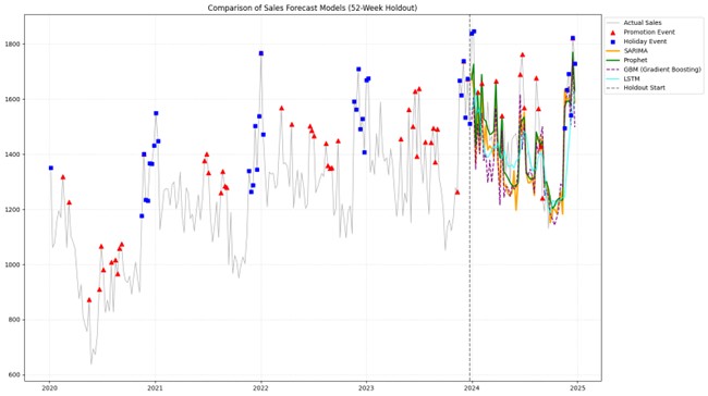
Common patterns may include:
A technically advanced model underperforming is not a failure. It is a design lesson.
Do not treat MAE as a winner label. A model with weaker average performance may still be valuable as a downside scenario, a challenger model, or an early-warning signal.
If the most adaptive model overshoots brief spikes, the error suggests sensitivity to transient noise. If the most stable model misses turning points, the error suggests delayed adaptation. Those errors mean different things for different decisions.
This SkillBox reinforces a core lesson of the chapter: AI-era forecasting is strongest when different model behaviors are interpreted as system inputs rather than forced into a single answer.
What kind of decision would make you prefer stability over responsiveness? What kind of decision would reverse that preference?
The next component moves from observing model behavior to reasoning with AI about disagreement, assumptions, and scenario framing.
Using AI as a Sensemaking Partner
This LearningLab reinforces the central idea of Chapter 7:
Forecasting is no longer about choosing the best model—it is about understanding how different models represent the system differently.
In the SkillBox, you implemented and compared multiple forecasting approaches (e.g., statistical models, machine learning models, and AI-driven methods).
This LearningLab uses AI as both a learning partner and a thinking partner to help you:
The objective is to:
This LearningLab reinforces:
AI is not used to select a model.
It is used to deepen your understanding of what each model contributes to the decision system.
In the SkillBox, you observed that different models can produce:
This raises a fundamental shift:
Model comparison is not about “which is best”—but about what each model reveals.
This LearningLab helps you move from:
AI is used here to:
Key principle:
Different models are not competitors—they are alternative representations of the same underlying system.
NorthStar analysts have implemented multiple forecasting approaches:
They observe:
This creates a critical question:
Which model should guide decisions—or should multiple models be used together?
Key questions include:
To address this, analysts use AI to:
AI does not determine which model is correct.
It helps you reason about how models differ—and why that matters.
You will engage with AI at three levels:
Reinforce → Extend → Explore
Work through the modes in order.
Strengthen your understanding of different forecasting paradigms.
“Key Concepts from Chapter 7.
“I understand how different models represent time series behavior differently.”
Extend your ability to evaluate and compare models analytically.
Optionally explore additional analytical concepts or methods that interest you but not covered in the chapter.
“I can critically compare models based on how they behave—not just how they score.”
Develop judgment by integrating multiple models into a decision system.
“I understand how multiple models can be combined to support better decisions.”
After completing all three modes:
The goal is to understand models as systems—not select winners.
Prepare a structured summary (200–300 words) including:
Your response should connect:
model behavior → interpretation → decision implication
You must:
Principle:
AI expands analytical range—but does not replace analytical judgment.
Different forecasting approaches encode structure differently:
These differences lead to:
No single model dominates across all conditions.
AI can:
But cannot:
Insight:
The value of multiple models lies not in agreement—but in the information revealed by their differences.
You have now moved from:
model comparison → model understanding → system thinking
The next step is:
designing how multiple models inform decisions
How should model outputs translate into:
The DesignStudio moves from:
understanding → reasoning → decision system design
This DesignStudio develops decision system design capability. Students move from comparing models to designing how those models should operate together within a governed forecasting process.
NorthStar Retail Group wants to modernize its forecasting capability. The company does not want to abandon classical forecasting, but it also recognizes that promotions, event signals, and shifting consumer behavior create situations where more adaptive models may add value. Leadership asks the analytics team to design a forecasting system that is faster and more flexible without becoming untrustworthy.
How should NorthStar design a hybrid forecasting system that balances:
NorthStar currently has:
A poorly governed system could either react too slowly to real shifts or overreact to noise. Both outcomes carry cost through inventory, staffing, promotion timing, and loss of managerial trust.
Design a governed forecasting system for NorthStar by addressing the following:
Submit a short system design memo or one-page framework that includes:
Responses are evaluated on decision structure, governance clarity, explicit trade-offs, and alignment with forecasting by design.
The strongest system is rarely the one with the most complex model. It is the one that makes complexity governable.
Where should NorthStar deliberately preserve visible structure even if a more complex model appears more adaptive?
The next component places this design logic into a different organizational context where leaders must act before uncertainty resolves.
A global streaming platform is planning its Q4 content release schedule and the associated infrastructure capacity needed to support it. Under ordinary conditions, demand is reasonably seasonal. But major content launches and social attention can create sharp, nonlinear surges across markets and time zones.
The analytics team has produced four forecasts for weekly global viewing demand using a classical model, a structured business forecasting model, a machine-learning model, and a deep-learning model. All were trained on the same historical data and evaluated over the same forecast horizon.
The forecasts do not agree.
Senior leadership must decide within two weeks whether to:
No one can wait until uncertainty resolves. A decision must be made now.
The forecasts suggest four different views of the future:
No forecast is obviously wrong. Each implies a different risk posture.
Submit one concise decision brief containing:
When models disagree, what matters more: choosing a winner or designing a decision that survives disagreement?
This case reinforces the core lesson of the chapter: when uncertainty is high, the challenge is not prediction alone. It is designing action that remains accountable across plausible futures.
AI does not replace forecasting structure; it changes where structure lives and how it must be governed. As forecasting systems become more adaptive, the analyst’s responsibility shifts from single-model selection to system design, validation, and scenario interpretation. In the age of AI, better forecasting means not only learning faster, but preserving accountability when forecasts shape decisions.
NorthStar Retail Group now sees forecasting as more than a sequence of models. The team has learned that classical baselines, adaptive challengers, and AI-assisted interpretation can each serve different roles within a governed system. Rather than asking which model is smartest, NorthStar is beginning to ask which configuration is most useful for planning, monitoring, and escalation. This marks an important shift from isolated forecasting techniques toward institutional forecasting capability. The company is now closer to treating forecasting as an organizational design discipline rather than a technical routine.
Explain reasoning clearly. Distinguish signal from noise. Connect analytical differences to decisions. Avoid purely technical answers that do not address interpretation, governance, or decision use.
Three ideas matter most in this chapter. First, AI does not remove forecasting structure; it relocates it from fully specified models toward features, learned representations, and governed systems. Second, different forecasting methods should be compared not only by accuracy, but by behavior, interpretability, and decision usefulness. Third, generative AI is most valuable as a sensemaking partner that helps teams interpret disagreement and organize scenarios without owning decisions.
One decision insight stands out: the best forecasting system is not the one with the most sophisticated algorithm, but the one that balances adaptability with accountability for the decision at hand.
One common mistake is to assume that more complex models are automatically better. In forecasting by design, complexity should be earned, monitored, and governed.
This chapter showed how AI expands forecasting systems, but it also revealed a deeper challenge: once multiple models, scenarios, and governance rules are in place, forecasting is no longer just an analytical workflow. It becomes an institutional capability. The next chapter therefore asks a broader question: how should organizations design forecasting not as a collection of methods, but as a disciplined system for decision-making, responsibility, and learning over time?

